We will go over several data transformations and standardizations (aka relativisations) commonly used in multivariate statistics. This material borrows heavily from Dr. Kevin McGarigals Applied Multivariate Course with some modifications here and there.
There are many packages out there (i.e, vegan) to automatically make these transformations but it is important to understand when and why we make these transformations and so next time you see that a function is doing a Wisconsin Double transformation, you know what just happened to your data.
A great reference that has considerably more detail about when and why to use these transformations can be found in Ecologically meaningful transformations for ordination of species data
What are the differences between Transformations and Standardizations?
-
Transformations are applied to each element of the data matrix, independent of the other elements
-
Standardizations adjust elements by a row or column statistic (e.g., max, sum, mean)
First we will go over Transformations and then to the Standardizations
Create some data
We will create a simple matrix that we will use as the basis for many of our transformations and standardizations
rawdata<-matrix(c(1,1,1,3,3,1,
                2,2,4,6,6,0,
                10,10,20,30, 30,0,
                3,3,2,1,1,0,
                0,0,0,0,1,0,
                0,0,0,0,20,0), 6, byrow =T)

rawdata
## [,1] [,2] [,3] [,4] [,5] [,6]
## [1,] 1 1 1 3 3 1
## [2,] 2 2 4 6 6 0
## [3,] 10 10 20 30 30 0
## [4,] 3 3 2 1 1 0
## [5,] 0 0 0 0 1 0
## [6,] 0 0 0 0 20 0Calculating row and column stats
In many of our standardizations, we will be manipulating each element in the matrix by a column and/or row statistics. Like most this in R, there are many ways to go about doing this.
Rows
# Sums
rowSums(rawdata)
## [1] 10 20 100 10 1 20apply(rawdata,1, sum)## [1] 10 20 100 10 1 20# Max values
apply(rawdata,1, max)## [1] 3 6 30 3 1 20Columns
# Sums
colSums(rawdata)
## [1] 16 16 27 40 61 1apply(rawdata,2, sum)## [1] 16 16 27 40 61 1# Max values
apply(rawdata,2, max)## [1] 10 10 20 30 30 1Monotonic transformations
Log transformations
- Useful when you have wide spread in the data.
- It is important that you add one to your values to account for zeros
log10(0+1) = 0)
To run this on the matrix, we can use the log10 function in base R. I like to get in the habitat of using the apply function, because I feel more certain in what the function is doing.
In using the apply function, we need to specify the direction. Above we saw that 1 was for rows and 2 was columns. Remember that when we are doing transformations, we need to apply these to each element. To specify this with apply we use c(1,2).
In addition, because we are going to add a value of 1 to each element, we need to specify function(x) in the apply statement. We will also be specifying this for any of the custom functions we will write.
logdata<-apply(rawdata,c(1,2), function(x) log10(x+1))

logdata
## [,1] [,2] [,3] [,4] [,5] [,6]
## [1,] 0.3010300 0.3010300 0.3010300 0.602060 0.602060 0.30103
## [2,] 0.4771213 0.4771213 0.6989700 0.845098 0.845098 0.00000
## [3,] 1.0413927 1.0413927 1.3222193 1.491362 1.491362 0.00000
## [4,] 0.6020600 0.6020600 0.4771213 0.301030 0.301030 0.00000
## [5,] 0.0000000 0.0000000 0.0000000 0.000000 0.301030 0.00000
## [6,] 0.0000000 0.0000000 0.0000000 0.000000 1.322219 0.00000To help visualize what this is doing, we will apply this the log10 tranformation on some data with a wide spread.
This data can be found here
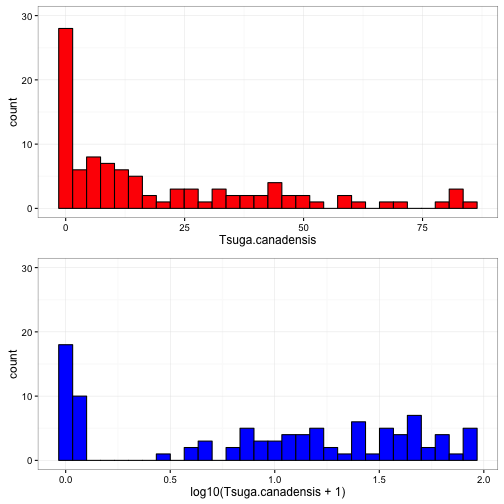
In the figure above, you can see that the values ranged 0, 85. The transformed data ranges 0, 1.93. With this transformation we have decreased the overall spread of the data.
Power transformations
- Square root transformation (trans = 2) most often used for Poisson data (i.e., count data).
- greater the value, greater the compression
- Flexible for a wide range of data
- Transformation is applied when x > 0.
To do this transformation we will write a function that will give us the ability to do several different power levels. In this function, we will have two parameters. x is the data to be transformed and trans will be power of the transformation (i.e., a trans of 2 will be a square root transformation $x^{1/2}$ )
pwr_trans<-function(x, trans){
  x<- ifelse(x>0,x^(1/trans),0)
  return(x)
}

pwr_trans(x = 16, trans = 2)
## [1] 4pwr_trans(x = 0, trans = 2)## [1] 0To illustrate how the level of the power influences the compression, we will use transformations of 2,3,4,5,10 of x values ranging from 1:100.
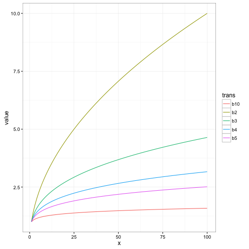
As can be observed above, as the level of the power increases the level of compression of the data decreases.
Presence absence transformations
- Transforms quantitative data to non-quantitative data
- Applicable to species data
- Most useful when there is not a lot of quantitative info present (lots of zeros or low abundances)
- Severe transformation: loose a lot of info
To do this transformation we will write a function that will change any x>0 to a 1. In this function, we will have one parameters. x is the data to be transformed.
pa_trans<-function(x){
  x<-ifelse(x>0,1,0)
  return(x)
  }

apply(rawdata,c(1,2), function(x) pa_trans(x))
## [,1] [,2] [,3] [,4] [,5] [,6]
## [1,] 1 1 1 1 1 1
## [2,] 1 1 1 1 1 0
## [3,] 1 1 1 1 1 0
## [4,] 1 1 1 1 1 0
## [5,] 0 0 0 0 1 0
## [6,] 0 0 0 0 1 0Arcsine transformations
Whenever I think of arcsine transformation, I think of this manuscript “The arcsine is asinine: the analysis of proportions in ecology”. Needless to say, that althought there are some strong feelings out there against using this transformation, I will go over it so that you know what it is doing.
- Transforms proportion data ($0 \ge x \le 1$)
- Useful for proportion data with a positive skew
- Spreads end of scale while compressing the middle
Before we apply the transformation we need to change our rawdata matrix into a proportion matrix. To do this we will do our first standardization and adjust each element by the row total (total number by site).
prop.data <- rawdata / apply(rawdata,1,sum)

# double check that we did it correctly
apply(prop.data,1,sum)
## [1] 1 1 1 1 1 1To do this transformation we will write a function that apply the arcsine transformation. In this function, we will have one parameters. x is the data to be transformed.
acsin_trans<-function(x){
  x<- 2/pi *asin(sqrt(x))
  return(x)
  }

apply(prop.data, c(1,2), function(x) acsin_trans(x))
## [,1] [,2] [,3] [,4] [,5] [,6]
## [1,] 0.2048328 0.2048328 0.2048328 0.3690101 0.3690101 0.2048328
## [2,] 0.2048328 0.2048328 0.2951672 0.3690101 0.3690101 0.0000000
## [3,] 0.2048328 0.2048328 0.2951672 0.3690101 0.3690101 0.0000000
## [4,] 0.3690101 0.3690101 0.2951672 0.2048328 0.2048328 0.0000000
## [5,] 0.0000000 0.0000000 0.0000000 0.0000000 1.0000000 0.0000000
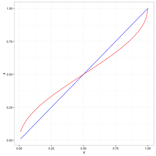
## [6,] 0.0000000 0.0000000 0.0000000 0.0000000 1.0000000 0.0000000To get a better idea, on how this transforms the data we will run it on a sequence of data between 0 and 1.
 In the figure above, our original data is indicated by the straight blue line and the red line is the transformed data. You can see that the values below
 0.50 are increased and the values above 0.50 were slightly decreased. Those values closer to extremes are changed more.
Standardizations
For the next few standardizations (max and sum) this can be applied to by both column and rows. There is only a slight difference in the way we apply the transformation to the matrix.
Sums
- Can be applied to any range of x
- Output will range 0 to 1
- Converts values to a relative value (equalizes the area under the curve)
- Used when there are differences in total abundance
Rows
When we were applying the arcsine transformation above we needed to construct the proportion. We did this by dividing each element in the matrix by the row sum.
rowprop.data <- rawdata / apply(rawdata,1,sum)

rowprop.data
## [,1] [,2] [,3] [,4] [,5] [,6]
## [1,] 0.1 0.1 0.1 0.3 0.3 0.1
## [2,] 0.1 0.1 0.2 0.3 0.3 0.0
## [3,] 0.1 0.1 0.2 0.3 0.3 0.0
## [4,] 0.3 0.3 0.2 0.1 0.1 0.0
## [5,] 0.0 0.0 0.0 0.0 1.0 0.0
## [6,] 0.0 0.0 0.0 0.0 1.0 0.0Columns
To standardize by columns we can not simply use the division symbol like we did with the rows. The reason has to do with matrix algebra that I am not going to get into here. If you would like a refresher on it check this page out.
To do this, we multiply rawdata by a matrix with the inverse of the column totals along the diagonal.
colprop.data <- rawdata %*% diag(1/apply(rawdata,2,sum))

colprop.data
## [,1] [,2] [,3] [,4] [,5] [,6]
## [1,] 0.0625 0.0625 0.03703704 0.075 0.04918033 1
## [2,] 0.1250 0.1250 0.14814815 0.150 0.09836066 0
## [3,] 0.6250 0.6250 0.74074074 0.750 0.49180328 0
## [4,] 0.1875 0.1875 0.07407407 0.025 0.01639344 0
## [5,] 0.0000 0.0000 0.00000000 0.000 0.01639344 0
## [6,] 0.0000 0.0000 0.00000000 0.000 0.32786885 0## double check to see if it was done correctly
apply(colprop.data,2,sum)## [1] 1 1 1 1 1 1For all the column transformations, we will use the same approach except changing the function in the apply statement.
Maximum
- Can be applied to any range of x
- Output will range 0 to 1, largest values will scale to 1
- Converts values to a relative value (equalizes the peak value)
- Used when there are differences in total abundance
Rows
rowmax.data <- rawdata / apply(rawdata,1,max)

rowmax.data
## [,1] [,2] [,3] [,4] [,5] [,6]
## [1,] 0.3333333 0.3333333 0.3333333 1.0000000 1.0000000 0.3333333
## [2,] 0.3333333 0.3333333 0.6666667 1.0000000 1.0000000 0.0000000
## [3,] 0.3333333 0.3333333 0.6666667 1.0000000 1.0000000 0.0000000
## [4,] 1.0000000 1.0000000 0.6666667 0.3333333 0.3333333 0.0000000
## [5,] 0.0000000 0.0000000 0.0000000 0.0000000 1.0000000 0.0000000
## [6,] 0.0000000 0.0000000 0.0000000 0.0000000 1.0000000 0.0000000Columns
colmax.data <- rawdata %*% diag(1/apply(rawdata,2,max))

colmax.data
## [,1] [,2] [,3] [,4] [,5] [,6]
## [1,] 0.1 0.1 0.05 0.10000000 0.10000000 1
## [2,] 0.2 0.2 0.20 0.20000000 0.20000000 0
## [3,] 1.0 1.0 1.00 1.00000000 1.00000000 0
## [4,] 0.3 0.3 0.10 0.03333333 0.03333333 0
## [5,] 0.0 0.0 0.00 0.00000000 0.03333333 0
## [6,] 0.0 0.0 0.00 0.00000000 0.66666667 0To illustrate what these standardizations are doing, we can look at the hypothetical abundance data for two species with different total abundance (sp.a = 100, sp.b = 200).
set.seed(1234)
spdat<-data.frame(spp= rep(c("sp.a","sp.b"), c(100,200)), N = c(rpois(100, 1),rpois(200, 5)))

spdata.summ<-spdat %>%
              group_by(spp, N) %>%
              summarise(ttl=n()) %>%
              ungroup() %>%
              complete(N, nesting(spp),fill=list(ttl = 0))

a<-ggplot(data=spdata.summ) +
  geom_bar(aes(x =N, y = ttl, fill=spp), position="dodge", stat="identity", colour="black", width = 1) +
  labs(y = "Frequency", x = "Count", title="Raw") +
  theme_bw() +
  theme(legend.position = c(0.94,0.55))

spdata.summ2<- spdata.summ %>%
                group_by(spp) %>%
                mutate(MaxN= max(ttl),
                       TTL = sum(ttl))

b<-ggplot(data=spdata.summ2) +
  geom_bar(aes(x =N, y = ttl/TTL, fill=spp), position="dodge", stat="identity", colour="black", width = 1) +
  labs(y = "Frequency", x = "Count", title="Column Total Standardization") +
  theme_bw() +
  theme(legend.position = "none")

c<-ggplot(data=spdata.summ2) +
  geom_bar(aes(x =N, y = ttl/MaxN, fill=spp), position="dodge", stat="identity", colour="black", width = 1) +
  labs(y = "Frequency", x = "Count", title="Column Max Standardization") +
  theme_bw() +
  theme(legend.position = "none")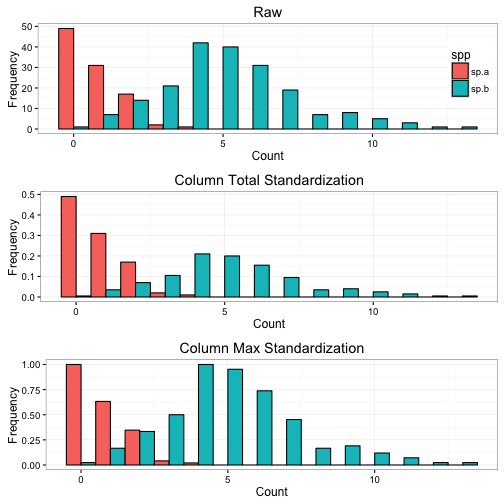
We can see that the standardizations have changed the distribution in the histograms. The total standardization equalized the area under the curve (if you add up the bars both equal 1), whereas the max equalized the max peaks in the graph (both equal 1).
Z-score standardization
- Can be applied to any range of x
- Output can be any value
- Converts values to z scores (mean = 0, variance = 1)
- Commonly used to put variables on equal scaling
- Important to use when you variables that are at different scales or units of measurement
- Tend to standardize across sites (i.e., by columns)
To do this transformation, we subtract each element by the column mean and then divide by the column standard deviation. The result is a value representing the number of standard deviations from the mean.
mvals<-apply(rawdata, 2, mean)
sdvals<-apply(rawdata, 2, sd)

std_data<-(rawdata - mvals) %*% diag(1 /sdvals)
std_data
## [,1] [,2] [,3] [,4] [,5]
## [1,] -0.44125282 -0.44125282 -0.21534527 0.02859712 0.02764689
## [2,] -0.17650113 -0.17650113 0.17227622 0.28597119 0.27646893
## [3,] 1.45613430 1.45613430 2.00271102 2.18767962 2.11498730
## [4,] -0.97075620 -0.97075620 -0.60296676 -0.48615103 -0.46999718
## [5,] -2.69164219 -2.69164219 -1.31360615 -0.87221213 -0.76028955
## [6,] -0.04412528 -0.04412528 -0.02153453 -0.01429856 1.64499012
## [,6]
## [1,] -4.0824829
## [2,] -6.5319726
## [3,] -11.0227038
## [4,] -16.3299316
## [5,] -24.9031457
## [6,] -0.4082483Normalization
- Can be applied to any range of x
- Output will range between 0 and 1
- Important to use when some rows have large variance and some small
- Common standardization in Principal Component Analysis (PCA)
In this standardization, each element is divided by its row minimum and then divided by the row range.
row.max<-apply(rawdata,1,max)
row.min<-apply(rawdata,1,min)

norm_data <- (rawdata - row.min)/(row.max - row.min)
norm_data
## [,1] [,2] [,3] [,4] [,5] [,6]
## [1,] 0.0000000 0.0000000 0.0000000 1.0000000 1.0000000 0
## [2,] 0.3333333 0.3333333 0.6666667 1.0000000 1.0000000 0
## [3,] 0.3333333 0.3333333 0.6666667 1.0000000 1.0000000 0
## [4,] 1.0000000 1.0000000 0.6666667 0.3333333 0.3333333 0
## [5,] 0.0000000 0.0000000 0.0000000 0.0000000 1.0000000 0
## [6,] 0.0000000 0.0000000 0.0000000 0.0000000 1.0000000 0Hellinger standardization
- Can be applied to any range of x
- Output will be any value but tend to be below 1
- Similar to the relativization by site
- Hellinger distance has good statistical properties as assessed by the criteria of R2 and monotonicity used by Legendre and Gallagher (2001)
In this standardization, each element is divided by its row sum. After the square root of each element is calculated.
hell_data <- sqrt(rawdata / apply(rawdata,1,sum))

hell_data
## [,1] [,2] [,3] [,4] [,5] [,6]
## [1,] 0.3162278 0.3162278 0.3162278 0.5477226 0.5477226 0.3162278
## [2,] 0.3162278 0.3162278 0.4472136 0.5477226 0.5477226 0.0000000
## [3,] 0.3162278 0.3162278 0.4472136 0.5477226 0.5477226 0.0000000
## [4,] 0.5477226 0.5477226 0.4472136 0.3162278 0.3162278 0.0000000
## [5,] 0.0000000 0.0000000 0.0000000 0.0000000 1.0000000 0.0000000
## [6,] 0.0000000 0.0000000 0.0000000 0.0000000 1.0000000 0.0000000Wisconsin Double standardization
- Can be applied to value of x > 0
- Output will range between 0 and 1
- Equalize emphasis among sample units and among species
- Difficult to understand individual data values after standardization
In this standardization, each element is divided by its column maximum and then divided by the row total
col.max<-apply(rawdata,2,max)

wdt_data.1 <- rawdata %*% diag(1 /col.max)

row.ttl<-apply(wdt_data.1,1,sum)

wdt_data <- wdt_data.1 / row.ttl

wdt_data
## [,1] [,2] [,3] [,4] [,5] [,6]
## [1,] 0.06896552 0.06896552 0.03448276 0.06896552 0.06896552 0.6896552
## [2,] 0.20000000 0.20000000 0.20000000 0.20000000 0.20000000 0.0000000
## [3,] 0.20000000 0.20000000 0.20000000 0.20000000 0.20000000 0.0000000
## [4,] 0.39130435 0.39130435 0.13043478 0.04347826 0.04347826 0.0000000
## [5,] 0.00000000 0.00000000 0.00000000 0.00000000 1.00000000 0.0000000
## [6,] 0.00000000 0.00000000 0.00000000 0.00000000 1.00000000 0.0000000Chi square standardization
- Can be applied to any range of x
- Output will be any value but tend to be below 1
- Used when you would like to give more weight to rarer species
In this standardization, each element is divided by its row sum and the square root of the column sum and multipled by the square root of the matrix sum.
row.sum<-apply(rawdata,1,sum)
col.sum<-apply(rawdata,2,sum)
mat.sum<- sum(rawdata)

chisq_data <- (rawdata / row.sum) %*% diag(1 /sqrt(col.sum)) * sqrt(mat.sum)

chisq_data
## [,1] [,2] [,3] [,4] [,5] [,6]
## [1,] 0.3172144 0.3172144 0.2441918 0.6018721 0.4873818 1.268858
## [2,] 0.3172144 0.3172144 0.4883836 0.6018721 0.4873818 0.000000
## [3,] 0.3172144 0.3172144 0.4883836 0.6018721 0.4873818 0.000000
## [4,] 0.9516433 0.9516433 0.4883836 0.2006240 0.1624606 0.000000
## [5,] 0.0000000 0.0000000 0.0000000 0.0000000 1.6246059 0.000000
## [6,] 0.0000000 0.0000000 0.0000000 0.0000000 1.6246059 0.000000Now that we have gone through all of this, the decostand function in the vegan package (as mentioned at the very top) can calculate these standardizations and transformations.