Background
The backbone to multivariate analysis is the two-way data matrix. In an ecological sense, we can imagine that each column in the dataset is a species or environmental factor and each row is a site. In a human dimensions sense, we can imagine a similar dataset where the columns are are responses to a question and each row is an individual.
This dataset can be be represented in an n-dimensional space based on its values within this data set. The points in that n-dimensional space form a data cloud. A primary goal of multivariate statistics is to describe the orientation of the points in this cloud.
For simplicity sake lets envision, a dataset with 4 sites (rows) and only 2 species (columns). The number of species A will be represented on the X axis and the number of species B will be represented on the Y axis.
library(ggplot2)

hyp_data<- matrix(c(1,9,1,8,6,6,9,1), byrow=TRUE, ncol = 2)
  colnames(hyp_data)<-c("SpeciesA","SpeciesB")

  ggplot(data=as.data.frame(hyp_data)) +
    geom_point(aes(x = SpeciesA, y = SpeciesB), size = 4, colour = "red") +
    geom_text(aes(x = SpeciesA, y = SpeciesB, label = paste("Site",1:4)), hjust = -0.25) +
    coord_cartesian(xlim = c(0, 10), ylim = c(0,10), expand = F) +
    theme_bw()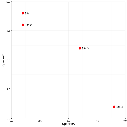
Now if you could imagine adding a third species, we would adjust the location of the sites along a third axis representing the number of species. The same goes for adding more and more species.
Similarity among sites
Most multivariate analysis uses similarities (or dissimilarities) to describe how each site (or individual) relates to the others based on species composition (or collective answers to questions).
Similarity
- Similarity is a characterization of the attributes in common compared to the total attributes.
- Sites with exactly the same attributes with have a similarity of 1, sites with no attributes the same will have a similarity of 0.
Dissimilarity
- Complement to similarity (i.e., 1 - similarity)
Distances
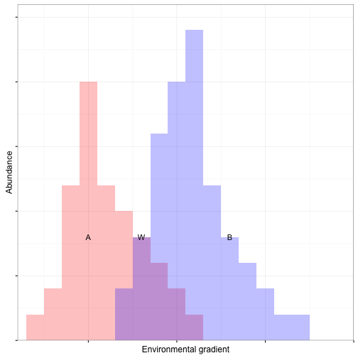
If we go back to our plot of the two species across four sites from earlier, we can visualize how similarity and distances are related. The visual layout of how these sites exist in the n-dimensional space can be thought of like a map. Points close together are more similar than points further away.
  ggplot(data=as.data.frame(hyp_data)) +
    geom_point(aes(x = SpeciesA, y = SpeciesB), size = 4, colour = "red") +
  geom_segment(data = as.data.frame(hyp_data)[-2,], aes(xend = SpeciesA, yend = SpeciesB, x = 1, y = 8), linetype="dashed" ) +
    geom_text(aes(x = SpeciesA, y = SpeciesB, label = paste("Site",1:4)), hjust = -0.25) +
    coord_cartesian(xlim = c(0, 10), ylim = c(0,10), expand = F) +
    theme_bw()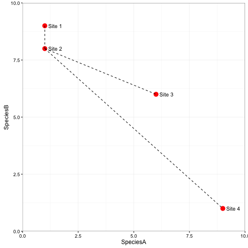
In the above plot, the dashed lines represent the distances between sites 1, 3, and 4 to site 2. Site 4 and Site 2 are the most different. If you look at the species composition you can see why. Site 2 had 1 of species A and 8 of Species B, whereas Site 4 had 9 of species A and 1 of species B. Sites 1 and 2 are the most similar. Site 2 had 1 of species A and 8 of Species B and Site 1 had 1 of species A and 9 of species B.
Distances are dissimilarities (dissimilarity = 1-similarity), or there are specific distance measures (e.g., Euclidean) that have no counterpart in similarity index.
Distances based on dissimilarites are bounded between 0 and 1. Distances based on a specific distance measures are unbounded.
The dimensions of the dissimilarity matrix are related to the number of rows in the 2-way data matrix.
dim(hyp_data)## [1] 4 2dist(hyp_data, diag=TRUE)## 1 2 3 4
## 1 0.000000
## 2 1.000000 0.000000
## 3 5.830952 5.385165 0.000000
## 4 11.313708 10.630146 5.830952 0.000000As you can see above, we had 4 sites so our distance matrix is a 4x4 matrix (the distance from each site to every site). The diagonal of the distance matrix should be 0 because it represents the comparison of each site to itself.
There are around 30 measures of similarities or distances (Legendre & Legendre 2012). The choice on which one to use will be related to the type of data that you have, the question, and the analysis.
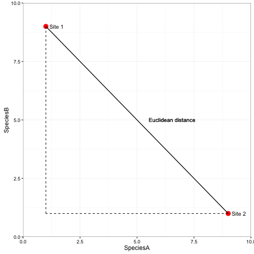
Euclidian distance
- Most appealing measure because it has true ‘metric’ properties
- Column standardized to remove issues with scale
- Applied to any data of any scale
- Used in eigenvector ordinations (e.g., PCA)
- Assumes variables are uncorrelated
- Emphasizes outliers
- Looses sensitivity with heterogeneous data
- Distances not proportional
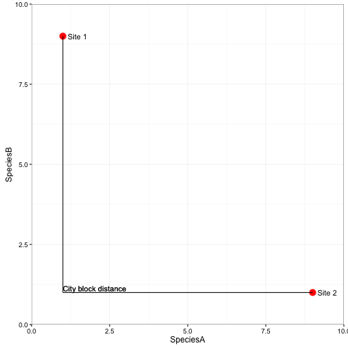
City-block (Manhattan) distance
- Most ecologically meaningful dissimilarities are Manhattan type
- Less weight to outliers compared to ED
- Retains sensitivity with heterogenous data
- Distances not proportional
Proportional Distances
- Manhattan distances expressed as a proportion to max distance
- 2 communities with nothing in common would have dissimilarity of 1
Sorensen or Bray-Curtis distance
- Percent dissimilarity
- Common with species data but can be used on any scale
- Gives less weight to outliers compared to ED
- Retains sensitivity with heterogeneous data
- Maximum when there is no shared species
- NOT metric and cannot be used with DA or CCA
A few other proportional distances exist and differ in how they weight the dissimilarity. Two examples are:
- Jaccard distance
- Kulcynski distance
Euclidean distances based on species profiles
Chord distance
- Similar conceptually to ED, but data are row normalized
- Useful in species abundance data because it removes differences in abundance
hyp_data3<- matrix(c(1,9,1,8,1,6,10,0,10,2,10,0), byrow=TRUE, ncol = 2)
  colnames(hyp_data3)<-c("SpeciesA","SpeciesB")

hyp_data3
## SpeciesA SpeciesB
## [1,] 1 9
## [2,] 1 8
## [3,] 1 6
## [4,] 10 0
## [5,] 10 2
## [6,] 10 0ss<-sqrt(apply(hyp_data3^2,1,sum)) # sqrt of (SpeciesA^2 + SpeciesB^2)
norm_data<-hyp_data3/ss
norm_data## SpeciesA SpeciesB
## [1,] 0.1104315 0.9938837
## [2,] 0.1240347 0.9922779
## [3,] 0.1643990 0.9863939
## [4,] 1.0000000 0.0000000
## [5,] 0.9805807 0.1961161
## [6,] 1.0000000 0.0000000dist(norm_data, "euclidean")## 1 2 3 4 5
## 2 0.01369767
## 3 0.05448471 0.04079085
## 4 1.33384292 1.32360513 1.29274979
## 5 1.18050527 1.16942057 1.13608606 0.19707524
## 6 1.33384292 1.32360513 1.29274979 0.00000000 0.19707524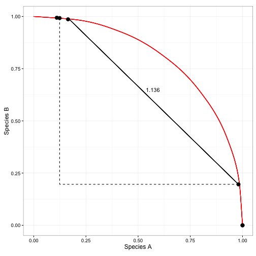
Chi-square distance
- ED after completing a row chi-quare standardization see last weeks notes
hyp_data3## SpeciesA SpeciesB
## [1,] 1 9
## [2,] 1 8
## [3,] 1 6
## [4,] 10 0
## [5,] 10 2
## [6,] 10 0row.sum<-apply(hyp_data3,1,sum)
col.sum<-apply(hyp_data3,2,sum)
mat.sum<- sum(hyp_data3)
chisq_data <- (hyp_data3 / row.sum) %*% diag(1 /sqrt(col.sum)) * sqrt(mat.sum)
chisq_data## [,1] [,2]
## [1,] 0.1325736 1.3708392
## [2,] 0.1473040 1.3539152
## [3,] 0.1893908 1.3055611
## [4,] 1.3257359 0.0000000
## [5,] 1.1047799 0.2538591
## [6,] 1.3257359 0.0000000dist(chisq_data, "euclidean")## 1 2 3 4 5
## 2 0.02243668
## 3 0.08654146 0.06410479
## 4 1.81737073 1.79493405 1.73082926
## 5 1.48082059 1.45838392 1.39427913 0.33655013
## 6 1.81737073 1.79493405 1.73082926 0.00000000 0.33655013Species-profile distance
- ED on relative abundances see last weeks notes
hyp_data3## SpeciesA SpeciesB
## [1,] 1 9
## [2,] 1 8
## [3,] 1 6
## [4,] 10 0
## [5,] 10 2
## [6,] 10 0row.sum<-apply(hyp_data3,1,sum)
prop_data <- (hyp_data3 / row.sum)
prop_data## SpeciesA SpeciesB
## [1,] 0.1000000 0.9000000
## [2,] 0.1111111 0.8888889
## [3,] 0.1428571 0.8571429
## [4,] 1.0000000 0.0000000
## [5,] 0.8333333 0.1666667
## [6,] 1.0000000 0.0000000dist(prop_data, "euclidean")## 1 2 3 4 5
## 2 0.01571348
## 3 0.06060915 0.04489567
## 4 1.27279221 1.25707872 1.21218305
## 5 1.03708995 1.02137646 0.97648079 0.23570226
## 6 1.27279221 1.25707872 1.21218305 0.00000000 0.23570226Hellinger distances
- ED on the Hellinger standardization see last weeks notes
hyp_data3## SpeciesA SpeciesB
## [1,] 1 9
## [2,] 1 8
## [3,] 1 6
## [4,] 10 0
## [5,] 10 2
## [6,] 10 0row.sum<-apply(hyp_data3,1,sum)
hell_data <- sqrt(hyp_data3 / row.sum)
hell_data## SpeciesA SpeciesB
## [1,] 0.3162278 0.9486833
## [2,] 0.3333333 0.9428090
## [3,] 0.3779645 0.9258201
## [4,] 1.0000000 0.0000000
## [5,] 0.9128709 0.4082483
## [6,] 1.0000000 0.0000000dist(hell_data, "euclidean")## 1 2 3 4 5
## 2 0.01808611
## 3 0.06583424 0.04775524
## 4 1.16942057 1.15470054 1.11537933
## 5 0.80501743 0.78842820 0.74431545 0.41744238
## 6 1.16942057 1.15470054 1.11537933 0.00000000 0.41744238Phew!! After going through all of these standardizations, transformations, and you have got to be thinking there has to be an easier way. And of course there is. The vegan package that I mentioned in the previous class has functions that will allow us to do all of these standardizations and distance measures. For example to run the
chi.sq transformation and the euclidean distance, we combine the use of the functions decostand (completes many of the common standardizations) and vegdist (completes many of the common distance measures).
library(vegan)

vegdist(decostand(hyp_data3, "chi.sq"), "euclidean")
## 1 2 3 4 5
## 2 0.02243668
## 3 0.08654146 0.06410479
## 4 1.81737073 1.79493405 1.73082926
## 5 1.48082059 1.45838392 1.39427913 0.33655013
## 6 1.81737073 1.79493405 1.73082926 0.00000000 0.33655013There are many other distance metrics we could choose from. Look at the help menu for vegdist (?vegdist) to get a better idea of what is available and how it is calculated.