Themes
One of my favorite aspects of ggplot2 is the use of themes. Not including a theme, the default ggplots theme is the theme_grey which has a dark grey background with white grid lines. See the example below
library(tidyverse)

 p<- ggplot(diamonds, ) +
      geom_point(aes(x=carat, y = price,colour=cut))
p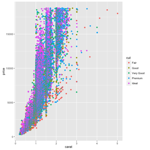
You see these plots all over the web and in presentations now and you can recognize the ggplot2 style.
There are a several “canned” themes that come with ggplot that offer themes do change the way the plot looks without having to edit every aspect of the visual presentation of the plot
theme_bw()
The classic dark-on-light ggplot2 theme. May work better for presentations displayed with a projector.
p + theme_bw()
theme_linedraw()
A theme with only black lines of various widths on white backgrounds, reminiscent of a line drawings. Serves a purpose similar to theme_bw. Note that this theme has some very thin lines (« 1 pt) which some journals may refuse.
p + theme_linedraw()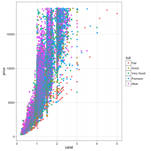
theme_light()
A theme similar to
theme_linedrawbut with light grey lines and axes, to direct more attention towards the data.
p + theme_light()
theme_minimal()
A minimalistic theme with no background annotations.
p + theme_minimal()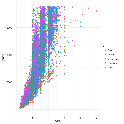
theme_classic()
A classic-looking theme, with x and y axis lines and no gridlines.
p + theme_classic()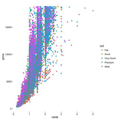
theme_dark()
The dark cousin of theme_light, with similar line sizes but a dark background. Useful to make thin coloured lines pop out.
p + theme_dark()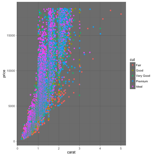
theme_void()
A completely empty theme.
p + theme_void()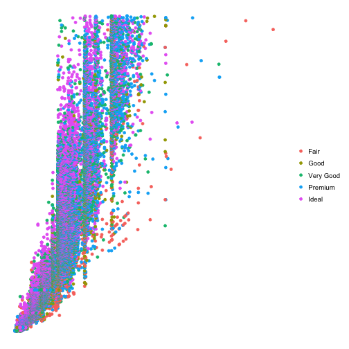
The problem with the default theme in ggplot is that these do not work for presentation formats (e.g., publication in a journal or presentation).
Other themes
There are lots of themes available online in various places. There is also the package ggthemes that offers many different themes and scales for graphics. Check out the gallery here.
There is also the ggthemr package
Making your own theme
While the theme_bw() is ok it does not meet publication quality figures (atleast in my field) or my typical presentation format. The great thing about ggplot is the ability to customize and create your own themes.
I have a few that I use on a regular basis The basic process is fairly straight forward. You start with the theme_bw and modify using %+replace% the aspects you wish to change (you do not need to specify all aspects).
theme_mine
theme_mine is the theme I use most often and is what I generally use for pubs.
theme_mine <- function(base_size = 18, base_family = "Helvetica") {
  # Starts with theme_grey and then modify some parts
  theme_bw(base_size = base_size, base_family = base_family) %+replace%
    theme(
      strip.background = element_blank(),
      strip.text.x = element_text(size = 18),
      strip.text.y = element_text(size = 18),
      axis.text.x = element_text(size=14),
      axis.text.y = element_text(size=14,hjust=1),
      axis.ticks =  element_line(colour = "black"),
      axis.title.x= element_text(size=16),
      axis.title.y= element_text(size=16,angle=90),
      panel.background = element_blank(),
      panel.border =element_blank(),
      panel.grid.major = element_blank(),
      panel.grid.minor = element_blank(),
      panel.margin = unit(1.0, "lines"),
      plot.background = element_blank(),
      plot.margin = unit(c(0.5,  0.5, 0.5, 0.5), "lines"),
      axis.line.x = element_line(color="black", size = 1),
        axis.line.y = element_line(color="black", size = 1)
    )
}


ggplot(diamonds) +
  geom_point(aes(x=carat, y = price,colour=cut)) +
  labs(title="theme_mine") +
  theme_mine()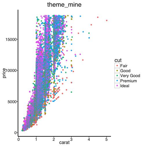
theme_presentation
My general format in presentations is to have a black background with white, yellow, and green text. I therefore created a theme (theme_presentation)that would work with the required black background and white text.
theme_presentation<- function(base_size = 28, base_family = "") {
  # Starts with theme_grey and then modify some parts
  theme_bw(base_size = base_size, base_family = base_family) %+replace%
    theme(
      strip.background = element_blank(),
      strip.text.x = element_text(size = 18,colour="white"),
      strip.text.y = element_text(size = 18,colour="white"),
      axis.text.x = element_text(size=28,colour="white"),
      axis.text.y = element_text(size=28,colour="white",hjust=1),
      axis.ticks =  element_line(colour = "white"),
      axis.title.x= element_text(size=42,colour="white"),
      axis.title.y= element_text(size=42,angle=90,colour="white"),
      panel.background = element_rect(fill="black"),
      panel.border =element_blank(),
      panel.grid.major = element_blank(),
      panel.grid.minor = element_blank(),
      panel.margin = unit(1.0, "lines"),
      plot.background = element_rect(fill="black"),
      plot.title =element_text(size=28,colour="white"),
      plot.margin = unit(c(1,  1, 1, 1), "lines"),
      legend.background=element_rect(fill='black'),
      legend.title=element_text(size=28,colour="white"),
      legend.text=element_text(size=28,colour="white"),
      legend.key = element_rect( fill = 'black'),
      legend.key.size = unit(c(1, 1), "lines"),
      axis.line.x = element_line(color="white", size = 1),
        axis.line.y = element_line(color="white", size = 1)
    )
}


ggplot(diamonds) +
  geom_point(aes(x=carat, y = price,colour=cut)) +
  labs(title="theme_presentation") +
  theme_presentation() +
  theme(legend.position=c(1,0.25))
## Warning in pmax(key_height, apply(key_sizes, 1, max)): an argument will be
## fractionally recycled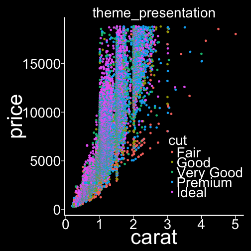
theme_map
I do a lot of map creation using ggplot and therefore the canned themes and the previous themes I discussed do not really fit. So I created a theme (theme_map).
library(maps)

theme_map <- function(base_size = 12, base_family = "") {
  # Starts with theme_grey and then modify some parts
  theme_bw(base_size = base_size, base_family = base_family) %+replace%
    theme(
      strip.background = element_blank(),
      strip.text.x = element_text(size = 18),
      strip.text.y = element_text(size = 18),
      axis.text.x = element_blank(),
      axis.text.y = element_blank(),
      axis.ticks = element_blank(),
      axis.title.x = element_blank(),
      axis.title.y = element_blank(),
      panel.background = element_blank(),
      panel.border =element_blank(),
      panel.grid.major = element_blank(),
      panel.grid.minor = element_blank(),
      panel.margin = unit(1.0, "lines"),
      plot.background = element_blank(),
      plot.margin = unit(c(0.25,  0.5, 0.0, 0.00), "lines"),
      axis.line = element_blank(),
      legend.background=element_blank(),
      legend.margin = unit(0.1, "line"),
      legend.title=element_text(size=16,colour="black"),
      legend.text=element_text(size=16,colour="black",hjust=0.2),
      legend.key = element_blank(),
      legend.key.width=unit(2, "line"),
      legend.key.height=unit(2, "line"))

}

crimes <- data.frame(state = tolower(rownames(USArrests)), USArrests)
states_map <- map_data("state")


ggplot(crimes, aes(map_id = state)) +
    geom_map(aes(fill = Murder), map = states_map) +
    labs(title="theme_map") +
    expand_limits(x = states_map$long, y = states_map$lat) +
    coord_map() +
    theme_map()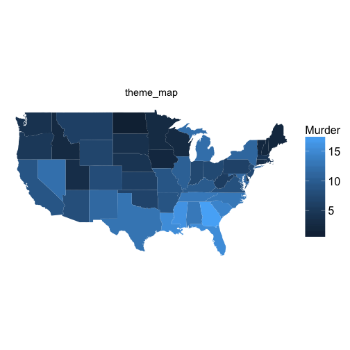
These files are included in a single file I call themes.r which I load as a source file in the housekeeping section of my R code.
Faceting
Faceting is the process of combining several plots together in a single figure. ggplot has two means of doing this, facet_grid and facet_wrap. I saw in a recent post that the ggplot2 version 2.2 will have a major revamp of facets.
facet_grid()
Lay out panels in a grid.
ggplot(data = mpg) +
  geom_point(aes(x = displ, y = cty))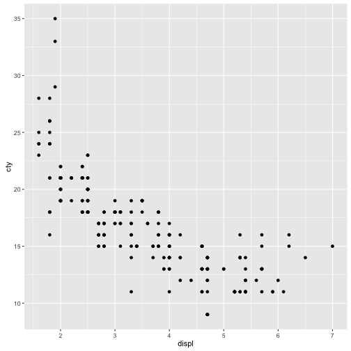
ggplot(data = mpg) +
  geom_point(aes(x = displ, y = cty)) +
  facet_grid(. ~ cyl)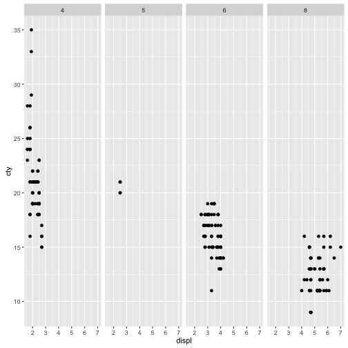
ggplot(data = mpg) +
  geom_point(aes(x = displ, y = cty)) +
  facet_grid(drv ~ .)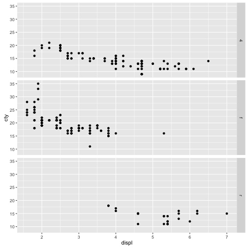
ggplot(data = mpg) +
  geom_point(aes(x = displ, y = cty)) +
  facet_grid(drv ~ cyl)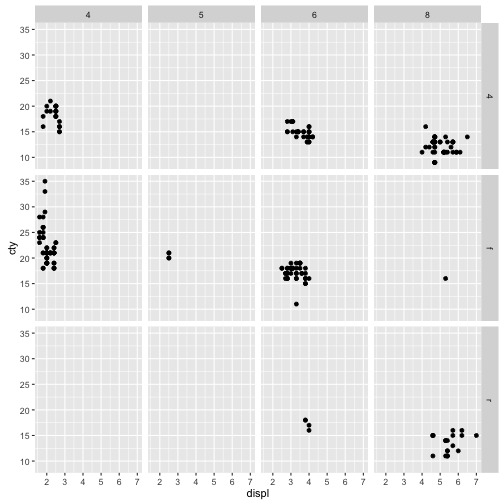
Messing with a few options in facet_grid
scales and space
ggplot(data = mtcars) +
  geom_point(aes(mpg, wt, colour = factor(cyl))) +
  facet_grid(. ~ cyl, scales = "free")
ggplot(data = mtcars) +
  geom_point(aes(mpg, wt, colour = factor(cyl))) +
  facet_grid(. ~ cyl, scales = "free_x")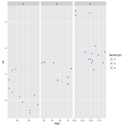
ggplot(data = mtcars) +
  geom_point(aes(mpg, wt, colour = factor(cyl))) +
  facet_grid(. ~ cyl, scales = "free_y")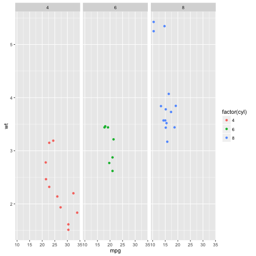
## space
ggplot(data = mpg) +
  geom_point(aes(drv, model)) +
  facet_grid(manufacturer ~ ., scales = "free", space = "free")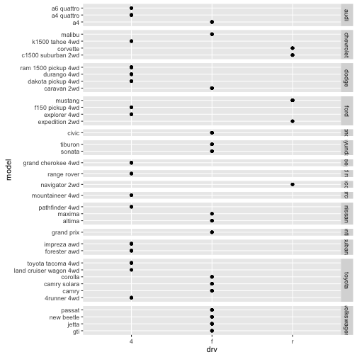
facet labels
# label_both() displays both variable name and value
 ggplot(data =mtcars) +
   geom_point(aes(wt, mpg), colour = "red") +
   facet_grid(vs ~ cyl, labeller = label_both)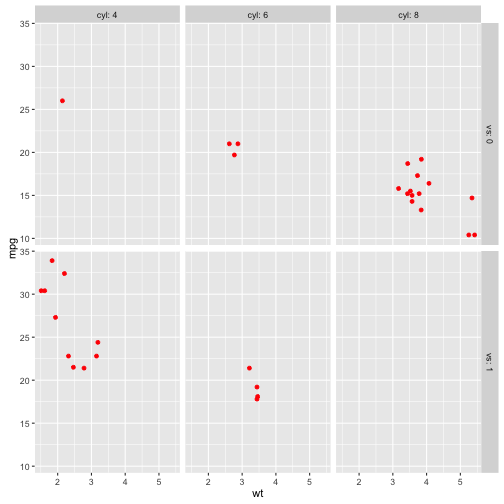
# Using label_parsed, see ?plotmath for more options
mtcars$cyl2 <- factor(mtcars$cyl, labels = c("beta", "gamma", "sqrt(x,y)"))

ggplot(data = mtcars) +
  geom_point(aes(wt, mpg), colour = "red") +
  facet_grid(. ~ cyl2)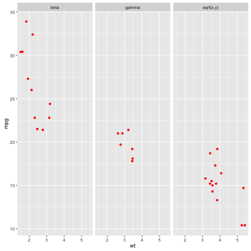
ggplot(data = mtcars) +
  geom_point(aes(wt, mpg), colour = "red") +
  facet_grid(. ~ cyl2, labeller = label_parsed)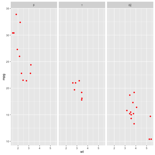
# label_bquote() makes it easy to construct math expressions
ggplot(data = mtcars) +
  geom_point(aes(wt, mpg), colour = "red") +
  facet_grid(. ~ vs, labeller = label_bquote(cols = alpha ^ .(vs)))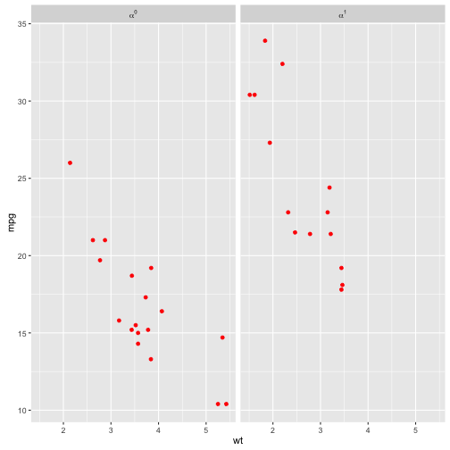
margins
ggplot(data = mtcars) +
  geom_point(aes(wt, mpg), colour = "red")  +
  facet_grid(vs + am ~ gear, margins = TRUE)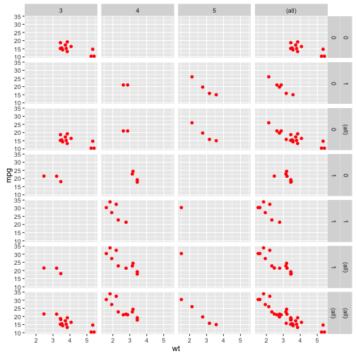
ggplot(data = mtcars) +
  geom_point(aes(wt, mpg), colour = "red")  +
  facet_grid(vs + am ~ gear, margins = "gear")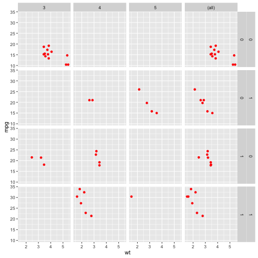
facet_wrap()
Lay out one dimension ribbon of panels into two dimensions. Many of the options in facet_grid are the same in facet_wrap.
ggplot(data = mpg) +
  geom_point(aes(x = displ, y = hwy), colour = "green") +
  facet_wrap(~ class)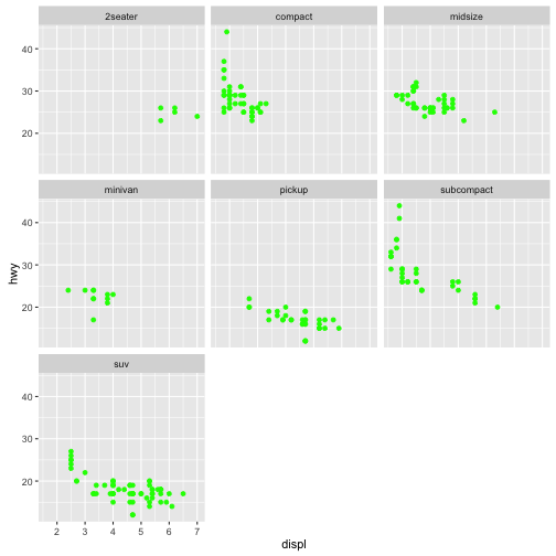
ggplot(data = mpg) +
  geom_point(aes(x = displ, y = hwy), colour = "green") +
  facet_wrap(~ class, ncol = 2)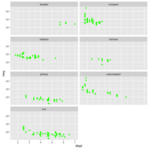
ggplot(data = mpg) +
  geom_point(aes(x = displ, y = hwy), colour = "green") +
  facet_wrap(~ class, nrow = 4)
ggplot(data = mpg) +
  geom_point(aes(x = displ, y = hwy), colour = "green") +
  facet_wrap(~ cyl + drv, nrow = 4)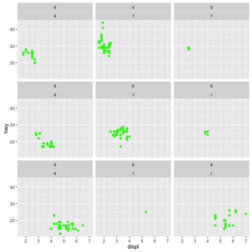
ggplot(data = mpg) +
  geom_point(aes(x = displ, y = hwy), colour = "green") +
  facet_wrap(~ cyl + drv, scales = "free")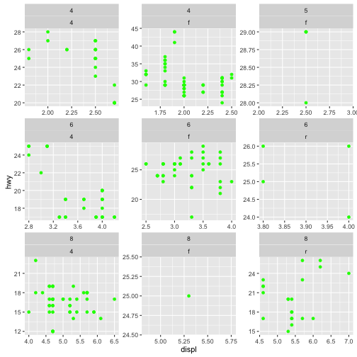
gridExtra
#install.packages(gridExtra)
library(gridExtra)

fake_data <- data.frame(x = 1:20)
fake_data$y <- fake_data$x * 0.3 + rnorm(20, sd = 2)

fake_data2 <- data.frame(x = 1:20)
fake_data2$y <- fake_data2$x * 3 + rnorm(20, sd = 6)


plota<-ggplot(data = fake_data) +
        geom_line(aes(x = x, y = y), colour = "red", linetype = "dashed") +
  theme(axis.title.y = element_blank(),
         axis.title.x = element_blank())

plotb<-ggplot(data = fake_data2) +
  geom_line(aes(x = x, y = y), colour = "blue", linetype = "dotted") +
  theme(axis.title.y = element_blank(),
         axis.title.x = element_blank())


grid.arrange(plota,plotb, ncol = 1, left = textGrob("Y", gp = gpar(fontsize = 18), rot = 90),
             bottom =textGrob("X", gp = gpar(fontsize = 18)) )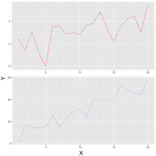
Notice that in the above plot, the two figures do not exactly line up. This takes a little finagling.
gA <- ggplotGrob(plota)
gB <- ggplotGrob(plotb)

maxWidth = grid::unit.pmax(gA$widths[2:5], gB$widths[2:5])
gA$widths[2:5] <- as.list(maxWidth)
gB$widths[2:5] <- as.list(maxWidth)

grid.arrange(gA, gB, ncol = 1, left = textGrob("Y", gp = gpar(fontsize = 18), rot = 90), bottom =textGrob("X", gp = gpar(fontsize = 18)))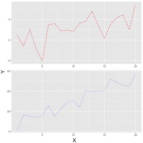
Outputting plots
You have two options when you are trying to output a plot.
Check out the options ?ggsave
 p<- ggplot(diamonds, ) +
      geom_point(aes(x=carat, y = price,colour=cut))

p

ggsave(filename = "path/to/where/you/want/your/file.png", dpi = 600, device = "png")
The other option that I use, particularly when you want to change the background color.
Check out the options using ?png
png(filename = "path/to/where/you/want/your/file.png")
  print(p)
dev.off()