This is just a gentle introduction to what you can do with Rmarkdown. There are lots of tutorials out there to help you further (Software carpentry, Data carpentry). There is also a lot more you can do with it than I have shown here. For example, you can alter the look of your html using CSS. In addition, given the limitation of the computers in the lab (i.e., no MikeTEX), we are going to limit ourselves to html this lesson. This should provide you a basic background to start creating your own documents.
Text modification
Italics
To do this you wrap the text you want italicized with _ or *.
Example: Lorem ipsum dolor sit amet,
Example: Lorem ipsum dolor sit amet,
Bold
To do this you wrap the text you want bold with **.
Example: vidisse vivendo est in,
Bold and italics
To do this you wrap the text you want bold and italicized with **_ your text _**.
Example: nam ea wisi similique.
Changing color
To change the color of the text is a litle more complicated, you will need to use <span style="color:yourcolor"</span .
Example: Per ne alienum tractatos. or Ne cum diceret postulant pertinacia.
Bulk quote
To do this you will need to use > followed by a hard break to stop.
Sit ullum delicata disputando ea. Te eam modo exerci nostrud, mei mandamus recteque ei. Quo at epicurei neglegentur, pro cu vitae constituto, at eum nulla electram euripidis. Et altera partiendo ius, no usu elit meliore oporteat. In tibique sententiae qui, cum affert viderer eu.
Subscripts and superscripts
You can create subscripts by using ~ ~ and supercripts by using ^ ^. For example,
F~2~ produces F~2~ and F^2^ produces F^2^.
Math equations
You can produce inline equations using $ $ or \\(. NOTE: If you are going to use inline equations on a github page you will need to use \\(. Writing mathematical equations will require some knowledge of Latex but it is generally easy to search and find what you need.
For example $E = mc^2$ produces $E = mc^2$ and \\( E = mc^2 \\) produces \( E = mc^2 \)
To create stand alone equations, you will use $$. NOTE: you can use $$ on github markdown pages. For example, $$y = \mu + \sum_{i=1}^p \beta_i x_i + \epsilon$$ produces
Creating lists
You can create bulleted lists by using a - or *. NOTE: sub-bullets must be indented 5 spaces in.
Idque conclusionemque sed et,
- et possim fierent posidonium nam.
- Enim petentium ex mei.
- Pertinacia mediocritatem eam ut,
- his iusto ullamcorper ex,
- eos id tota voluptua.
You can create numbered lists by using 1.
- et possim fierent posidonium nam.
- Enim petentium ex mei.
And the number order is not overly important. It will increase your list by units of one from the number at the top of your list.
- et possim fierent posidonium nam.
- Enim petentium ex mei.
And you can combine numbers and bullets:
- et possim fierent posidonium nam.
- Enim petentium ex mei.
- Pertinacia mediocritatem eam ut,
- his iusto ullamcorper ex,
- eos id tota voluptua.
Links
Weblinks
You can link any text to a website by enclosing the text you would like to provide a link with [] with the link immediately encapsulated in (). NOTE: do not put a space between the two.
Example:
This is a link to my [website](http://chrischizinski.github.io/) will give you
This is a link to my website.
Figures
To include a figure you use: 
To a file path: 
or to a website: 
Working with the R in Rmarkdown
The beauty of Rmarkdown is the ability to work directly with R in your documents. These are completed by using chunks.
Chunks
Chunks can be added in a few different ways
You can quickly insert chunks like these into your file with
- the keyboard shortcut Ctrl + Alt + I (OS X: Cmd + Option + I)
- the Add Chunk command in the editor toolbar
- or by typing the chunk delimiters
{r} and.
The chunk delimiter: ` ```{r nameofchunk knitr options}`
Chunk Options
There are a lot of different ways to customize your chunks (knitr options). These different options are inserted in the chunk {}
include = FALSEprevents code and results from appearing in the finished file. R Markdown still runs the code in the chunk, and the results can be used by other chunks.
#  This chunk will show up in your document
a <- 2
b <- 3

a+b
## [1] 5message = FALSEprevents messages that are generated by code from appearing in the finished file.
message_function<-function(x){
  if(x<5) message("x is les than 5")
  if(x>6) warning("x greater than 6")
  return(x)
}

message_function(4)
## x is les than 5## [1] 4message_function(4)## [1] 4warning = FALSEprevents warnings that are generated by code from appearing in the finished.
message_function(10)## Warning in message_function(10): x greater than 6## [1] 10message_function(10)## [1] 10echo = FALSEprevents code, but not the results from appearing in the finished file. This is a useful way to embed figures.
# All your code shows up here
library(tidyverse)
p <- ggplot() + geom_point(data =mtcars, aes(x=wt, y=mpg))
p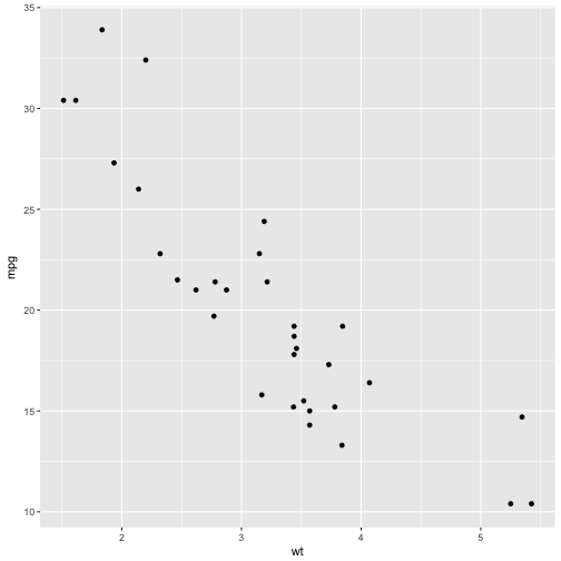
Only the results show up if you put echo = FALSE

fig.cap = "..."adds a caption to graphical results. See the R Markdown Reference Guide for a complete list of knitr chunk options.
Global Options
To set global options that apply to every chunk in your file, call knitr::opts_chunk$set in a code chunk. Knitr will treat each option that you pass to knitr::opts_chunk$set as a global default that can be overwritten in individual chunk headers.