Getting to know R again (with some new stuff thrown in)
Using data from Google sheets (kind of)
Google Forms is a quick and cheap way to put together an online survey. I asked you all to do the survey through Google Forms so that we can run some of the analysis with your responses. The survey responses were scrubbed of any individual information.
Getting data straight into used to be a bit more complicated but thanks to the googlesheets package it is a lot easier. NOTE: this does require you to accept some permissions before using with your individual account. Information on this can be found here.
Install googlesheets using:
install.packages('googlesheets')And then load the required libraries
library(googlesheets)
library(tidyverse)NOTE: googlesheets will not let me run the code but I will describe what is done below.
We can identify what google sheets are available on your googledrive by using the gs_ls() command.
gs_ls()  #  This displays the avaliable googlesheets on your google drive

ed <- gs_title("EcologicalDetective")  #  This registers the sheet "EcologicalDetective" so that we can read it in

survey_data <- gs_read(ss=ed)  # bring data in from google drive
Since the googlesheets will not work in a Rmarkdown environment, we can also read it in from github.
survey_data <- read_csv("https://raw.githubusercontent.com/chrischizinski/SNR_R_Group/master/data/EcologicalDetective.csv")## Parsed with column specification:
## cols(
## `Timestamp` = col_character(),
## `Name (First, Last)` = col_character(),
## `Do you plan to attend the group on a regular basis during the spring 2017 semester?` = col_character(),
## `How familiar are you with R?` = col_integer(),
## `How familiar are you with statistics?` = col_integer(),
## `Will you be using your own laptop? If NO, there are computers available in the lab` = col_character(),
## `If you are using your own laptop, is the most recent version of R (v 3.3.1 or greater) already installed on your computer?` = col_character(),
## `If you are using your own laptop, is the most recent version of RStudio (v 1.0 or greater) already installed on your computer?` = col_character(),
## `What R skills are you most interested in learning? [Inputting data into R]` = col_character(),
## `What R skills are you most interested in learning? [R data structures (arrays, matrices, data frames, lists)]` = col_character(),
## `What R skills are you most interested in learning? [Data wrangling]` = col_character(),
## `What R skills are you most interested in learning? [Data manipulation and summarization]` = col_character(),
## `What R skills are you most interested in learning? [Graphing]` = col_character(),
## `What R skills are you most interested in learning? [Report generation]` = col_character(),
## `Anything else not included above that you are interested in learning?` = col_character()
## )glimpse(survey_data)## Observations: 30
## Variables: 15
## $ Timestamp <chr> ...
## $ Name (First, Last) <chr> ...
## $ Do you plan to attend the group on a regular basis during the spring 2017 semester? <chr> ...
## $ How familiar are you with R? <int> ...
## $ How familiar are you with statistics? <int> ...
## $ Will you be using your own laptop? If NO, there are computers available in the lab <chr> ...
## $ If you are using your own laptop, is the most recent version of R (v 3.3.1 or greater) already installed on your computer? <chr> ...
## $ If you are using your own laptop, is the most recent version of RStudio (v 1.0 or greater) already installed on your computer? <chr> ...
## $ What R skills are you most interested in learning? [Inputting data into R] <chr> ...
## $ What R skills are you most interested in learning? [R data structures (arrays, matrices, data frames, lists)] <chr> ...
## $ What R skills are you most interested in learning? [Data wrangling] <chr> ...
## $ What R skills are you most interested in learning? [Data manipulation and summarization] <chr> ...
## $ What R skills are you most interested in learning? [Graphing] <chr> ...
## $ What R skills are you most interested in learning? [Report generation] <chr> ...
## $ Anything else not included above that you are interested in learning? <chr> ...As you can see above, the column headers are very long and messy. One way we can deal with that is to rename the headers, but we do want to preserve the original headings. We will do this by creating a new data.frame that has the new column name and the original column name.
survey_questions <- data.frame(new = c("Timestamp", paste("Q", 2:ncol(survey_data), sep="")), old = names(survey_data))

survey_questions
## new
## 1 Timestamp
## 2 Q2
## 3 Q3
## 4 Q4
## 5 Q5
## 6 Q6
## 7 Q7
## 8 Q8
## 9 Q9
## 10 Q10
## 11 Q11
## 12 Q12
## 13 Q13
## 14 Q14
## 15 Q15
## old
## 1 Timestamp
## 2 Name (First, Last)
## 3 Do you plan to attend the group on a regular basis during the spring 2017 semester?
## 4 How familiar are you with R?
## 5 How familiar are you with statistics?
## 6 Will you be using your own laptop? If NO, there are computers available in the lab
## 7 If you are using your own laptop, is the most recent version of R (v 3.3.1 or greater) already installed on your computer?
## 8 If you are using your own laptop, is the most recent version of RStudio (v 1.0 or greater) already installed on your computer?
## 9 What R skills are you most interested in learning? [Inputting data into R]
## 10 What R skills are you most interested in learning? [R data structures (arrays, matrices, data frames, lists)]
## 11 What R skills are you most interested in learning? [Data wrangling]
## 12 What R skills are you most interested in learning? [Data manipulation and summarization]
## 13 What R skills are you most interested in learning? [Graphing]
## 14 What R skills are you most interested in learning? [Report generation]
## 15 Anything else not included above that you are interested in learning?And then rename the survey_data with the new column names.
names(survey_data) <- survey_questions$new
glimpse(survey_data)
## Observations: 30
## Variables: 15
## $ Timestamp <chr> "1/9/2017 9:42:15", "1/9/2017 9:42:55", "1/9/2017 9:...
## $ Q2 <chr> "XXXX", "XXXX", "XXXX", "XXXX", "XXXX", "XXXX", "XXX...
## $ Q3 <chr> "No", "Yes", "Yes", "Yes", "Maybe", "Maybe", "Maybe"...
## $ Q4 <int> NA, 7, 4, 2, 3, 2, 3, 2, 4, 2, NA, NA, 5, 8, NA, 4, ...
## $ Q5 <int> NA, 7, 4, 4, 7, 7, 3, 1, 2, 6, NA, NA, 5, 4, NA, 4, ...
## $ Q6 <chr> NA, "Yes", "Yes", "No", "Maybe", "No", "Yes", "Maybe...
## $ Q7 <chr> NA, "Yes", "Yes", NA, "No, but I will have it done p...
## $ Q8 <chr> NA, "Yes", "Yes", NA, "No, but I will have it done p...
## $ Q9 <chr> NA, "Least interested", "Least interested", "Neutral...
## $ Q10 <chr> NA, "Least interested", "Neutral", "Most interested"...
## $ Q11 <chr> NA, "Most interested", "Interested", "Most intereste...
## $ Q12 <chr> NA, "Most interested", "Interested", "Most intereste...
## $ Q13 <chr> NA, "Neutral", "Most interested", "Most interested",...
## $ Q14 <chr> NA, "Most interested", "Most interested", "Intereste...
## $ Q15 <chr> NA, "Multivariate stats!", NA, NA, NA, "All of it. I...Messing with dates and times
Anyone that has tried using dates and times in R, has usually run into a giant headache at one time. The primary difficulty I always had is remembering and then typing out the correct format so that the character string can be parsed into the correct units of time.
survey_data$Timestamp## [1] "1/9/2017 9:42:15" "1/9/2017 9:42:55" "1/9/2017 9:44:51"
## [4] "1/9/2017 9:46:20" "1/9/2017 9:46:47" "1/9/2017 9:53:11"
## [7] "1/9/2017 9:54:19" "1/9/2017 9:55:30" "1/9/2017 9:58:05"
## [10] "1/9/2017 10:04:55" "1/9/2017 10:20:39" "1/9/2017 10:22:05"
## [13] "1/9/2017 10:26:41" "1/9/2017 10:47:34" "1/9/2017 11:00:12"
## [16] "1/9/2017 11:01:50" "1/9/2017 11:09:46" "1/9/2017 11:35:20"
## [19] "1/9/2017 11:36:22" "1/9/2017 11:38:32" "1/9/2017 11:55:06"
## [22] "1/9/2017 12:27:19" "1/9/2017 13:07:34" "1/9/2017 13:39:57"
## [25] "1/9/2017 14:35:05" "1/10/2017 9:48:46" "1/10/2017 10:07:21"
## [28] "1/10/2017 14:28:32" "1/11/2017 10:45:02" "1/12/2017 10:19:30"class(survey_data$Timestamp)## [1] "character"test <- as.POSIXlt(survey_data$Timestamp, format = "%m/%d/%Y %H:%M:%S")
test## [1] "2017-01-09 09:42:15 CST" "2017-01-09 09:42:55 CST"
## [3] "2017-01-09 09:44:51 CST" "2017-01-09 09:46:20 CST"
## [5] "2017-01-09 09:46:47 CST" "2017-01-09 09:53:11 CST"
## [7] "2017-01-09 09:54:19 CST" "2017-01-09 09:55:30 CST"
## [9] "2017-01-09 09:58:05 CST" "2017-01-09 10:04:55 CST"
## [11] "2017-01-09 10:20:39 CST" "2017-01-09 10:22:05 CST"
## [13] "2017-01-09 10:26:41 CST" "2017-01-09 10:47:34 CST"
## [15] "2017-01-09 11:00:12 CST" "2017-01-09 11:01:50 CST"
## [17] "2017-01-09 11:09:46 CST" "2017-01-09 11:35:20 CST"
## [19] "2017-01-09 11:36:22 CST" "2017-01-09 11:38:32 CST"
## [21] "2017-01-09 11:55:06 CST" "2017-01-09 12:27:19 CST"
## [23] "2017-01-09 13:07:34 CST" "2017-01-09 13:39:57 CST"
## [25] "2017-01-09 14:35:05 CST" "2017-01-10 09:48:46 CST"
## [27] "2017-01-10 10:07:21 CST" "2017-01-10 14:28:32 CST"
## [29] "2017-01-11 10:45:02 CST" "2017-01-12 10:19:30 CST"class(test)## [1] "POSIXlt" "POSIXt"Luckily, the lubridate package has come along that has greatly simplified the process of dealing with dates and times. lubridate will parse out your data using typical characters (“/” or “-“ and it will tell you if it can’t figure them out), if you provide the order that your date is formatted.
library(lubridate)##
## Attaching package: 'lubridate'## The following object is masked from 'package:base':
##
## date# ymd() year month day
# dmy() day month year
# hms() hours minutes seconds
# ymd_hms() year month day hours minutes seconds
# dmy_hm day month year hours minutes
# and so on
# As an example using our survey data
mdy_hms(survey_data$Timestamp, tz = "America/Chicago")## [1] "2017-01-09 09:42:15 CST" "2017-01-09 09:42:55 CST"
## [3] "2017-01-09 09:44:51 CST" "2017-01-09 09:46:20 CST"
## [5] "2017-01-09 09:46:47 CST" "2017-01-09 09:53:11 CST"
## [7] "2017-01-09 09:54:19 CST" "2017-01-09 09:55:30 CST"
## [9] "2017-01-09 09:58:05 CST" "2017-01-09 10:04:55 CST"
## [11] "2017-01-09 10:20:39 CST" "2017-01-09 10:22:05 CST"
## [13] "2017-01-09 10:26:41 CST" "2017-01-09 10:47:34 CST"
## [15] "2017-01-09 11:00:12 CST" "2017-01-09 11:01:50 CST"
## [17] "2017-01-09 11:09:46 CST" "2017-01-09 11:35:20 CST"
## [19] "2017-01-09 11:36:22 CST" "2017-01-09 11:38:32 CST"
## [21] "2017-01-09 11:55:06 CST" "2017-01-09 12:27:19 CST"
## [23] "2017-01-09 13:07:34 CST" "2017-01-09 13:39:57 CST"
## [25] "2017-01-09 14:35:05 CST" "2017-01-10 09:48:46 CST"
## [27] "2017-01-10 10:07:21 CST" "2017-01-10 14:28:32 CST"
## [29] "2017-01-11 10:45:02 CST" "2017-01-12 10:19:30 CST"# A few other examples
mdy_hms("Jan 1 2017 12:00:00")## [1] "2017-01-01 12:00:00 UTC"mdy_hms("January 1, 2017 12:00:00")## [1] "2017-01-01 12:00:00 UTC"mdy_hms("1-1,2017 12:00:00")## [1] "2017-01-01 12:00:00 UTC"# Write the formatting to our data
survey_data$Timestamp <- mdy_hms(survey_data$Timestamp, tz = "America/Chicago")
#And take a look
glimpse(survey_data)## Observations: 30
## Variables: 15
## $ Timestamp <dttm> 2017-01-09 09:42:15, 2017-01-09 09:42:55, 2017-01-0...
## $ Q2 <chr> "XXXX", "XXXX", "XXXX", "XXXX", "XXXX", "XXXX", "XXX...
## $ Q3 <chr> "No", "Yes", "Yes", "Yes", "Maybe", "Maybe", "Maybe"...
## $ Q4 <int> NA, 7, 4, 2, 3, 2, 3, 2, 4, 2, NA, NA, 5, 8, NA, 4, ...
## $ Q5 <int> NA, 7, 4, 4, 7, 7, 3, 1, 2, 6, NA, NA, 5, 4, NA, 4, ...
## $ Q6 <chr> NA, "Yes", "Yes", "No", "Maybe", "No", "Yes", "Maybe...
## $ Q7 <chr> NA, "Yes", "Yes", NA, "No, but I will have it done p...
## $ Q8 <chr> NA, "Yes", "Yes", NA, "No, but I will have it done p...
## $ Q9 <chr> NA, "Least interested", "Least interested", "Neutral...
## $ Q10 <chr> NA, "Least interested", "Neutral", "Most interested"...
## $ Q11 <chr> NA, "Most interested", "Interested", "Most intereste...
## $ Q12 <chr> NA, "Most interested", "Interested", "Most intereste...
## $ Q13 <chr> NA, "Neutral", "Most interested", "Most interested",...
## $ Q14 <chr> NA, "Most interested", "Most interested", "Intereste...
## $ Q15 <chr> NA, "Multivariate stats!", NA, NA, NA, "All of it. I...There are also several helper functions that will help you retrieve various bits of information associated with the dates and times
hour(survey_data$Timestamp) # Retrieves the hour## [1] 9 9 9 9 9 9 9 9 9 10 10 10 10 10 11 11 11 11 11 11 11 12 13
## [24] 13 14 9 10 14 10 10minute(survey_data$Timestamp) # Retrieves the minute## [1] 42 42 44 46 46 53 54 55 58 4 20 22 26 47 0 1 9 35 36 38 55 27 7
## [24] 39 35 48 7 28 45 19second(survey_data$Timestamp) # Retrieves the second## [1] 15 55 51 20 47 11 19 30 5 55 39 5 41 34 12 50 46 20 22 32 6 19 34
## [24] 57 5 46 21 32 2 30year(survey_data$Timestamp) # Retrieves the year## [1] 2017 2017 2017 2017 2017 2017 2017 2017 2017 2017 2017 2017 2017 2017
## [15] 2017 2017 2017 2017 2017 2017 2017 2017 2017 2017 2017 2017 2017 2017
## [29] 2017 2017leap_year(survey_data$Timestamp) #TRUE/FALSE if the year is a leap year## [1] FALSE FALSE FALSE FALSE FALSE FALSE FALSE FALSE FALSE FALSE FALSE
## [12] FALSE FALSE FALSE FALSE FALSE FALSE FALSE FALSE FALSE FALSE FALSE
## [23] FALSE FALSE FALSE FALSE FALSE FALSE FALSE FALSEmonth(survey_data$Timestamp) # Retrieves the month## [1] 1 1 1 1 1 1 1 1 1 1 1 1 1 1 1 1 1 1 1 1 1 1 1 1 1 1 1 1 1 1day(survey_data$Timestamp) # Retrieves the day## [1] 9 9 9 9 9 9 9 9 9 9 9 9 9 9 9 9 9 9 9 9 9 9 9
## [24] 9 9 10 10 10 11 12wday(survey_data$Timestamp) # Retrieves the day of the week, numeric## [1] 2 2 2 2 2 2 2 2 2 2 2 2 2 2 2 2 2 2 2 2 2 2 2 2 2 3 3 3 4 5wday(survey_data$Timestamp, label = TRUE) # Retrieves the day of week, word## [1] Mon Mon Mon Mon Mon Mon Mon Mon Mon Mon Mon
## [12] Mon Mon Mon Mon Mon Mon Mon Mon Mon Mon Mon
## [23] Mon Mon Mon Tues Tues Tues Wed Thurs
## Levels: Sun < Mon < Tues < Wed < Thurs < Fri < Satyday(survey_data$Timestamp) # Retrieves the day of year## [1] 9 9 9 9 9 9 9 9 9 9 9 9 9 9 9 9 9 9 9 9 9 9 9
## [24] 9 9 10 10 10 11 12mday(survey_data$Timestamp) # Retrieves the day of month## [1] 9 9 9 9 9 9 9 9 9 9 9 9 9 9 9 9 9 9 9 9 9 9 9
## [24] 9 9 10 10 10 11 12We can even use lubridate to look at periods of time
email_sent <- mdy_hms("January 9, 2017 9:39:00",tz = "America/Chicago")
email_sent
## [1] "2017-01-09 09:39:00 CST"intv_data <- interval(email_sent, survey_data$Timestamp) # Create intervals between the timestamps of each survey and when I sent the email invitation
intv_data## [1] 2017-01-09 09:39:00 CST--2017-01-09 09:42:15 CST
## [2] 2017-01-09 09:39:00 CST--2017-01-09 09:42:55 CST
## [3] 2017-01-09 09:39:00 CST--2017-01-09 09:44:51 CST
## [4] 2017-01-09 09:39:00 CST--2017-01-09 09:46:20 CST
## [5] 2017-01-09 09:39:00 CST--2017-01-09 09:46:47 CST
## [6] 2017-01-09 09:39:00 CST--2017-01-09 09:53:11 CST
## [7] 2017-01-09 09:39:00 CST--2017-01-09 09:54:19 CST
## [8] 2017-01-09 09:39:00 CST--2017-01-09 09:55:30 CST
## [9] 2017-01-09 09:39:00 CST--2017-01-09 09:58:05 CST
## [10] 2017-01-09 09:39:00 CST--2017-01-09 10:04:55 CST
## [11] 2017-01-09 09:39:00 CST--2017-01-09 10:20:39 CST
## [12] 2017-01-09 09:39:00 CST--2017-01-09 10:22:05 CST
## [13] 2017-01-09 09:39:00 CST--2017-01-09 10:26:41 CST
## [14] 2017-01-09 09:39:00 CST--2017-01-09 10:47:34 CST
## [15] 2017-01-09 09:39:00 CST--2017-01-09 11:00:12 CST
## [16] 2017-01-09 09:39:00 CST--2017-01-09 11:01:50 CST
## [17] 2017-01-09 09:39:00 CST--2017-01-09 11:09:46 CST
## [18] 2017-01-09 09:39:00 CST--2017-01-09 11:35:20 CST
## [19] 2017-01-09 09:39:00 CST--2017-01-09 11:36:22 CST
## [20] 2017-01-09 09:39:00 CST--2017-01-09 11:38:32 CST
## [21] 2017-01-09 09:39:00 CST--2017-01-09 11:55:06 CST
## [22] 2017-01-09 09:39:00 CST--2017-01-09 12:27:19 CST
## [23] 2017-01-09 09:39:00 CST--2017-01-09 13:07:34 CST
## [24] 2017-01-09 09:39:00 CST--2017-01-09 13:39:57 CST
## [25] 2017-01-09 09:39:00 CST--2017-01-09 14:35:05 CST
## [26] 2017-01-09 09:39:00 CST--2017-01-10 09:48:46 CST
## [27] 2017-01-09 09:39:00 CST--2017-01-10 10:07:21 CST
## [28] 2017-01-09 09:39:00 CST--2017-01-10 14:28:32 CST
## [29] 2017-01-09 09:39:00 CST--2017-01-11 10:45:02 CST
## [30] 2017-01-09 09:39:00 CST--2017-01-12 10:19:30 CSTas.period(intv_data) # Convert to period## [1] "3M 15S" "3M 55S" "5M 51S" "7M 20S"
## [5] "7M 47S" "14M 11S" "15M 19S" "16M 30S"
## [9] "19M 5S" "25M 55S" "41M 39S" "43M 5S"
## [13] "47M 41S" "1H 8M 34S" "1H 21M 12S" "1H 22M 50S"
## [17] "1H 30M 46S" "1H 56M 20S" "1H 57M 22S" "1H 59M 32S"
## [21] "2H 16M 6S" "2H 48M 19S" "3H 28M 34S" "4H 0M 57S"
## [25] "4H 56M 5S" "1d 0H 9M 46S" "1d 0H 28M 21S" "1d 4H 49M 32S"
## [29] "2d 1H 6M 2S" "3d 0H 40M 30S"as.period(intv_data, unit = "s") # Specify seconds## [1] "195S" "235S" "351S" "440S" "467S" "851S" "919S"
## [8] "990S" "1145S" "1555S" "2499S" "2585S" "2861S" "4114S"
## [15] "4872S" "4970S" "5446S" "6980S" "7042S" "7172S" "8166S"
## [22] "10099S" "12514S" "14457S" "17765S" "86986S" "88101S" "103772S"
## [29] "176762S" "261630S"as.numeric(as.period(intv_data, unit = "s")) # convert that period to numeric so you can analyze## [1] 195 235 351 440 467 851 919 990 1145 1555
## [11] 2499 2585 2861 4114 4872 4970 5446 6980 7042 7172
## [21] 8166 10099 12514 14457 17765 86986 88101 103772 176762 261630as.numeric(as.period(intv_data, unit = "s"))/60 # Decimal minutes## [1] 3.250000 3.916667 5.850000 7.333333 7.783333
## [6] 14.183333 15.316667 16.500000 19.083333 25.916667
## [11] 41.650000 43.083333 47.683333 68.566667 81.200000
## [16] 82.833333 90.766667 116.333333 117.366667 119.533333
## [21] 136.100000 168.316667 208.566667 240.950000 296.083333
## [26] 1449.766667 1468.350000 1729.533333 2946.033333 4360.500000You can also use lubridate to add periods of time to dates and times
survey_data$Timestamp + days(2) # Add two days to all the times## [1] "2017-01-11 09:42:15 CST" "2017-01-11 09:42:55 CST"
## [3] "2017-01-11 09:44:51 CST" "2017-01-11 09:46:20 CST"
## [5] "2017-01-11 09:46:47 CST" "2017-01-11 09:53:11 CST"
## [7] "2017-01-11 09:54:19 CST" "2017-01-11 09:55:30 CST"
## [9] "2017-01-11 09:58:05 CST" "2017-01-11 10:04:55 CST"
## [11] "2017-01-11 10:20:39 CST" "2017-01-11 10:22:05 CST"
## [13] "2017-01-11 10:26:41 CST" "2017-01-11 10:47:34 CST"
## [15] "2017-01-11 11:00:12 CST" "2017-01-11 11:01:50 CST"
## [17] "2017-01-11 11:09:46 CST" "2017-01-11 11:35:20 CST"
## [19] "2017-01-11 11:36:22 CST" "2017-01-11 11:38:32 CST"
## [21] "2017-01-11 11:55:06 CST" "2017-01-11 12:27:19 CST"
## [23] "2017-01-11 13:07:34 CST" "2017-01-11 13:39:57 CST"
## [25] "2017-01-11 14:35:05 CST" "2017-01-12 09:48:46 CST"
## [27] "2017-01-12 10:07:21 CST" "2017-01-12 14:28:32 CST"
## [29] "2017-01-13 10:45:02 CST" "2017-01-14 10:19:30 CST"survey_data$Timestamp + seconds(30) # Add 30 seconds to all the times## [1] "2017-01-09 09:42:45 CST" "2017-01-09 09:43:25 CST"
## [3] "2017-01-09 09:45:21 CST" "2017-01-09 09:46:50 CST"
## [5] "2017-01-09 09:47:17 CST" "2017-01-09 09:53:41 CST"
## [7] "2017-01-09 09:54:49 CST" "2017-01-09 09:56:00 CST"
## [9] "2017-01-09 09:58:35 CST" "2017-01-09 10:05:25 CST"
## [11] "2017-01-09 10:21:09 CST" "2017-01-09 10:22:35 CST"
## [13] "2017-01-09 10:27:11 CST" "2017-01-09 10:48:04 CST"
## [15] "2017-01-09 11:00:42 CST" "2017-01-09 11:02:20 CST"
## [17] "2017-01-09 11:10:16 CST" "2017-01-09 11:35:50 CST"
## [19] "2017-01-09 11:36:52 CST" "2017-01-09 11:39:02 CST"
## [21] "2017-01-09 11:55:36 CST" "2017-01-09 12:27:49 CST"
## [23] "2017-01-09 13:08:04 CST" "2017-01-09 13:40:27 CST"
## [25] "2017-01-09 14:35:35 CST" "2017-01-10 09:49:16 CST"
## [27] "2017-01-10 10:07:51 CST" "2017-01-10 14:29:02 CST"
## [29] "2017-01-11 10:45:32 CST" "2017-01-12 10:20:00 CST"Manipulating and plotting the data
Let’s use dplyr and tidyr to manipulate the data
survey_data_rev <- survey_data %>%
                    select(-Q2) %>%  # remove Q2
                    arrange(Timestamp) %>% # order by the timestamp
                    mutate(TakeSurvey = 1,  # Create new column called TakeSurvey
                           cuml_Order = cumsum(TakeSurvey), # Calculate the cumulative sum
                           prop_Order = cuml_Order/sum(TakeSurvey))  # Calculate the cumulative proportion of when people took the survey

glimpse(survey_data_rev)
## Observations: 30
## Variables: 17
## $ Timestamp <dttm> 2017-01-09 09:42:15, 2017-01-09 09:42:55, 2017-01-...
## $ Q3 <chr> "No", "Yes", "Yes", "Yes", "Maybe", "Maybe", "Maybe...
## $ Q4 <int> NA, 7, 4, 2, 3, 2, 3, 2, 4, 2, NA, NA, 5, 8, NA, 4,...
## $ Q5 <int> NA, 7, 4, 4, 7, 7, 3, 1, 2, 6, NA, NA, 5, 4, NA, 4,...
## $ Q6 <chr> NA, "Yes", "Yes", "No", "Maybe", "No", "Yes", "Mayb...
## $ Q7 <chr> NA, "Yes", "Yes", NA, "No, but I will have it done ...
## $ Q8 <chr> NA, "Yes", "Yes", NA, "No, but I will have it done ...
## $ Q9 <chr> NA, "Least interested", "Least interested", "Neutra...
## $ Q10 <chr> NA, "Least interested", "Neutral", "Most interested...
## $ Q11 <chr> NA, "Most interested", "Interested", "Most interest...
## $ Q12 <chr> NA, "Most interested", "Interested", "Most interest...
## $ Q13 <chr> NA, "Neutral", "Most interested", "Most interested"...
## $ Q14 <chr> NA, "Most interested", "Most interested", "Interest...
## $ Q15 <chr> NA, "Multivariate stats!", NA, NA, NA, "All of it. ...
## $ TakeSurvey <dbl> 1, 1, 1, 1, 1, 1, 1, 1, 1, 1, 1, 1, 1, 1, 1, 1, 1, ...
## $ cuml_Order <dbl> 1, 2, 3, 4, 5, 6, 7, 8, 9, 10, 11, 12, 13, 14, 15, ...
## $ prop_Order <dbl> 0.03333333, 0.06666667, 0.10000000, 0.13333333, 0.1...Now plot the data
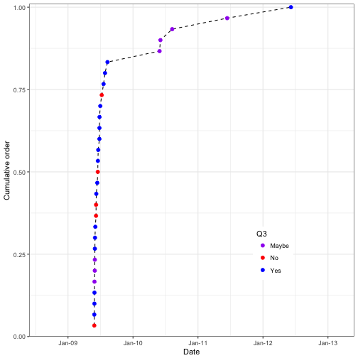
ggplot(data = survey_data_rev) +
  geom_line(aes(x = Timestamp, y = prop_Order), linetype = "dashed") + # Create dashed lines with x as Timestamp and y the cumulative proportion
  geom_point(aes(x = Timestamp, y = prop_Order, color = Q3), size = 2) + # Add points at each of the times
  labs(y = "Cumulative order", x = "Date") + #set the axis lables
  scale_color_manual(values = c("Maybe" = "purple", "Yes" = "blue", "No" = "red")) +  # Set the colours of the points
  theme_bw() + # Use the canned black and white theme
  theme(legend.position = c(0.75,0.25))  # Change the location of the legend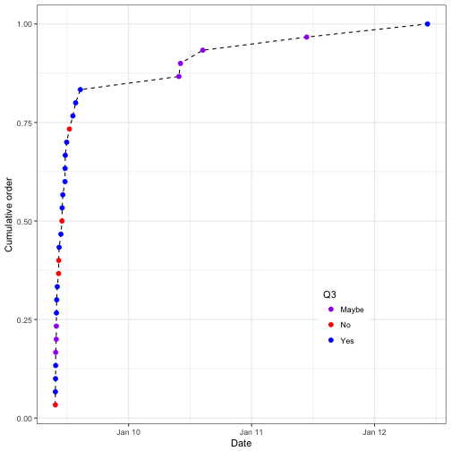
Adjust the x-axis with dates and times
library(scales)

email_sent
## [1] "2017-01-09 09:39:00 CST"time_stop <- email_sent + days(4) # Add four days past when the initial email was sent
ggplot(data = survey_data_rev) +
geom_line(aes(x = Timestamp, y = prop_Order), linetype = "dashed") +
geom_point(aes(x = Timestamp, y = prop_Order, color = Q3), size = 2) +
labs(y = "Cumulative order", x = "Date") +
coord_cartesian(ylim = c(0,1.01), expand = FALSE) +
scale_color_manual(values = c("Maybe" = "purple", "Yes" = "blue", "No" = "red")) +
scale_x_datetime(limits = c(email_sent - days(1), time_stop)) + #Set the date limits
theme_bw() +
theme(legend.position = c(0.75,0.25))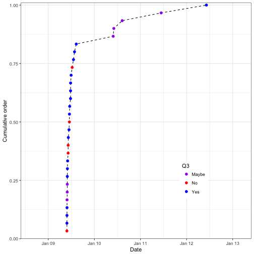
And add different breaks and date/time formatting
ggplot(data = survey_data_rev) +
  geom_line(aes(x = Timestamp, y = prop_Order), linetype = "dashed") +
  geom_point(aes(x = Timestamp, y = prop_Order, color = Q3), size = 2) +
  labs(y = "Cumulative order", x = "Date") +
  coord_cartesian(ylim = c(0,1.01), expand = FALSE) +
  scale_color_manual(values = c("Maybe" = "purple", "Yes" = "blue", "No" = "red")) +
  scale_x_datetime(limits = c(email_sent - days(1), time_stop), breaks = date_breaks("1 day"), labels = date_format("%b-%d")) +
  theme_bw() +
  theme(legend.position = c(0.75,0.25))