The RMarkdown file for this lesson can be found here.
This lesson will follow Chapter 8 in Quinn and Keough (2002).
Load the packages we will be using in this lesson
library(tidyverse)
library(broom)
library(lme4)
library(multcomp)
Comparing groups or treatments
- Analysis of variance (ANOVA) is a statistical technique to partition and analyze the variation of a continuous response variable
- Previously we used ANOVA to partition the variation in a response variable into that explained by the linear regression with one or more continuous predictor variables and that unexplained by the regression model
- The statistical distinction between “classical regression” and “classical ANOVA” is artificial, which is why we can use the
lm()withanova()or theaovfunction in R - Two prime reasons to use classical ANOVA:
- examine the relative contribution of sources of variation to the total amount of the variability in the response variable
- test the null hypothesis (H0) that population group or treatment means are equal
Single factor
- A single factor or one way design = single factor or predictor
- factor can comprise several levels
- completely randomized (CR) designs (no restriction on the random allocation of experimental or sampling units to factor levels)
Types of predictors
- Two types of factors
- Fixed - all the levels of the factor that are of interest are included in the analysis
- cannot extrapolate beyond these levels, repeat experiment keep same levels
- called: fixed effect models or Model 1 ANOVAs
- conclusions for a fixed factor are restricted to those specific groups we used in the experiment or sampling program
- Random - we are only using a random selection of all the possible levels of the factor
- usually make inferences about all the possible groups from our sample of groups
- called: random effect models or Model 2 ANOVAs
- analogous to Model 2 regression
- draw conclusions about the population of groups from which we have randomly chosen a subset (like site or time)
- Fixed - all the levels of the factor that are of interest are included in the analysis
Lets begin exploring this in R, using the medley data
This data includes:
- STREAM - name of streams in the Rocky Mountain region of Colorado, USA
- ZINC - categorical zinc concentration level (HIGH=high, MED=medium, LOW=low, BACK=background)
- DIVERSTY - Shannon-Wiener species diversity of diatoms
- ZNGROUP - alternative categorical zinc concentration level (1=background, 2=low, 3=medium, 4=high)
medley <- read_csv("https://raw.githubusercontent.com/chrischizinski/SNR_R_Group/master/data/ExperimentalDesignData/chpt08/medley.csv")## Parsed with column specification:
## cols(
## STREAM = col_character(),
## ZINC = col_character(),
## DIVERSTY = col_double(),
## ZNGROUP = col_integer(),
## RESID1 = col_double(),
## PREDICT1 = col_double(),
## RESID2 = col_double(),
## PREDICT2 = col_double()
## )glimpse(medley)## Observations: 34
## Variables: 8
## $ STREAM <chr> "Eagle", "Eagle", "Eagle", "Eagle", "Blue", "Blue", "...
## $ ZINC <chr> "BACK", "HIGH", "HIGH", "MED", "BACK", "HIGH", "BACK"...
## $ DIVERSTY <dbl> 2.27, 1.25, 1.15, 1.62, 1.70, 0.63, 2.05, 1.98, 1.04,...
## $ ZNGROUP <int> 1, 4, 4, 3, 1, 4, 1, 1, 4, 3, 3, 1, 3, 4, 4, 4, 2, 2,...
## $ RESID1 <dbl> 0.47250000, -0.02777778, -0.12777778, -0.09777778, -0...
## $ PREDICT1 <dbl> 1.797500, 1.277778, 1.277778, 1.717778, 1.797500, 1.2...
## $ RESID2 <dbl> 0.69750000, -0.32250000, -0.42250000, 0.04750000, 0.0...
## $ PREDICT2 <dbl> 1.572500, 1.572500, 1.572500, 1.572500, 1.670000, 1.6...medley %>%
mutate(ZINC = factor(ZINC, levels = c("BACK","LOW","MED","HIGH")),
AllDiversity = mean(DIVERSTY)) %>%
group_by(ZINC) %>%
summarise(MeanDiversity = mean(DIVERSTY),
SEDiversity = sd(DIVERSTY)/sqrt(length(DIVERSTY)),
ALLDiversity = mean(AllDiversity))## # A tibble: 4 × 4
## ZINC MeanDiversity SEDiversity ALLDiversity
## <fctr> <dbl> <dbl> <dbl>
## 1 BACK 1.797500 0.1715658 1.694118
## 2 LOW 2.032500 0.1573298 1.694118
## 3 MED 1.717778 0.1676701 1.694118
## 4 HIGH 1.277778 0.1422906 1.694118ANOVA - Fixed effects
med_mod <- lm(DIVERSTY ~ ZINC, data = medley)
summary (med_mod)
##
## Call:
## lm(formula = DIVERSTY ~ ZINC, data = medley)
##
## Residuals:
## Min 1Q Median 3Q Max
## -1.03750 -0.22896 0.07986 0.33222 0.79750
##
## Coefficients:
## Estimate Std. Error t value Pr(>|t|)
## (Intercept) 1.79750 0.16478 10.909 5.81e-12 ***
## ZINCHIGH -0.51972 0.22647 -2.295 0.0289 *
## ZINCLOW 0.23500 0.23303 1.008 0.3213
## ZINCMED -0.07972 0.22647 -0.352 0.7273
## ---
## Signif. codes: 0 '***' 0.001 '**' 0.01 '*' 0.05 '.' 0.1 ' ' 1
##
## Residual standard error: 0.4661 on 30 degrees of freedom
## Multiple R-squared: 0.2826, Adjusted R-squared: 0.2108
## F-statistic: 3.939 on 3 and 30 DF, p-value: 0.01756anova(med_mod)## Analysis of Variance Table
##
## Response: DIVERSTY
## Df Sum Sq Mean Sq F value Pr(>F)
## ZINC 3 2.5666 0.85554 3.9387 0.01756 *
## Residuals 30 6.5164 0.21721
## ---
## Signif. codes: 0 '***' 0.001 '**' 0.01 '*' 0.05 '.' 0.1 ' ' 1med_aov<-aov(DIVERSTY ~ ZINC, data = medley)
summary(med_aov)## Df Sum Sq Mean Sq F value Pr(>F)
## ZINC 3 2.567 0.8555 3.939 0.0176 *
## Residuals 30 6.516 0.2172
## ---
## Signif. codes: 0 '***' 0.001 '**' 0.01 '*' 0.05 '.' 0.1 ' ' 1Remember we can partition the total sum of squares \( SS_{T} \) can be partitioned into two components
-
ZINCrepresents variation due to the difference between group means - calculated as \( \bar{y_i} \) - \( \bar{y} \); df is the number of groups minus 1 Residualsdifference between the observations within each group- calculated as \( y_{ij} \) - \( \bar{y_i} \); df is sum of the sample sizes minus the number of groups
- The mean squares from the ANOVA are sample variances
- \( MS_{residuals} \) estimates \( \alpha_{\epsilon}^2 \) , the pooled population variance of the error terms within groups. (Assumes homogeneity of error variances)
- \( MS_{groups} \) estimates the pooled variance of the error terms across groups plus: - a component representing the squared effects of the chosen groups if the factor is fixed - the variance between all possible groups if the factor is random
Null hypothesis
- Fixed effects: the null hypothesis tested in a single factor ANOVA is usually one of no difference between group means or no effect of treatments
- Random effects: the null hypothesis is that the variance between all possible groups equals zero
If the H0 for a fixed factor is true, all \( \alpha_i \) equal zero (no group effects) and both \( MS_{groups} \) and \( MS_{residual} \) estimate \( \alpha_{\epsilon}^2 \) and their ratio should be one. The ratio of two variances (or mean squares) is called an F-ratio.
-
If the H0 is false, then at least one \( \alpha_i \) will be different from zero. Therefore, \( MS_{groups} \) has a larger expected value than \( MS_{residual} \) and their F-ratio will be greater than one.
-
A central F distribution is a probability distribution of the F-ratio when the two sample variances come from populations with the same expected values. There are different central F distributions depending on the df of the two sample variances
We can explore this using the df and F-value to show the probability calculation. df = 3, 30 and F-value = 3.9387
# Calculate the F-value
tidy_aov<-tidy(med_aov)
F_val<- tidy_aov$meansq[1]/tidy_aov$meansq[2]
F_val
## [1] 3.93869# Create a probability distribution
f_prob<-data.frame(F =seq(0,8, by = 0.1),pval= pf(seq(0,8, by = 0.1), 3, 30))
# Plot this distribution
ggplot(data = f_prob) +
geom_line(aes(x = F, y = pval)) +
geom_vline(aes(xintercept = 3.9387), colour = "red") +
annotate('text', x = 3.9387, y = 0.5, label = paste(round(1-pf(3.9387, 3, 30), digits = 4)), hjust = 0) +
theme_bw()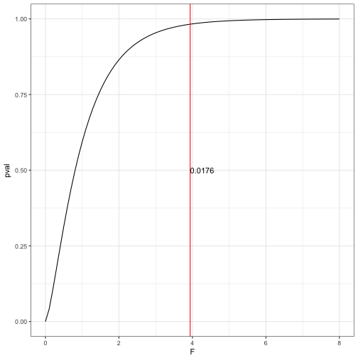
- Construction of the tests of null hypotheses is identical for fixed and random factors in the single factor ANOVA model but these null hypotheses have very different interpretations - The H0 for the fixed factor refers only to the groups used in the study whereas the H0 for the random factor refers to all the possible groups that could have been used - The assumption of equal within group variances is so important. For example, if \( \alpha_{i1} \) does not equal \( \alpha_{i2} \), then \( MS_{residual} \) does not estimate a single population variance , and we cannot construct a reliable F-ratio for testing the H0 of no group effects
Unbalanced designs
- Unequal sample sizes among groups can cause some problems: 1. Different group means will be estimated with different levels of precision, which can make interpretation difficult 2. ANOVA F test is more sensitive to violations of assumptions (i.e., homogeneity of variances) if sample sizes differ 3. Estimation of group effects is more difficult 4. Power calculations for random effects models are difficult
So what do you do if you have an unbalanced design?
- Delete observations to make it balanced
- Substitute group means to make balanced
- If differences in sample size and homogeneity of variances does not seem violated, fit linear ANOVA
- Prevent unbalanced designs in the experimental design
Factor effects
- In regression, with a continuous predictor, the coefficient value in the models is an assessment of the effect size of X on Y
- When your predictor is categorical how do we measure effect size? - One measure of group effects is the variance associated with the groups over and above the residual variance (similar to \( R^2 \))
tidy_aov$sumsq[1]/sum(tidy_aov$sumsq)## [1] 0.2825725glance(med_aov)$r.squared## [1] 0.2825725What can be some of the issues with this measure?
Random effects: variance components
- There are two variance components of interest
- true variance between replicate observations within each group, averaged across groups is estimated by \( MS_{residual} \) or \( \sigma_{\epsilon}^2 \)
- true variance between the means of all the possible groups we could have used in our study is is termed the added variance component due to groups \( \sigma_{a}^2 \)
Explore this lets make a balanced dataset
set.seed(12345)
n<-20
rand_effects_dat1 <- data.frame(GRP = "A",
                               Value = rnorm(n, mean= 15, sd = 3))
rand_effects_dat2 <- data.frame(GRP = "B",
                               Value = rnorm(n, mean= 30, sd = 3))
rand_effects_dat3 <- data.frame(GRP = "C",
                               Value = rnorm(n, mean= 20, sd = 3))
rand_effects_dat4 <- data.frame(GRP = "D",
                               Value = rnorm(n, mean= 45, sd = 3))

rand_effects_dat <- rbind(rand_effects_dat1,
                          rand_effects_dat2,
                          rand_effects_dat3,
                          rand_effects_dat4)

## Random effect ANOVA
aov_re<-aov(Value ~ Error(GRP), data = rand_effects_dat)

err_grp <- data.frame(unclass(summary(aov_re)$`Error: GRP`))
err_res <- data.frame(unclass(summary(aov_re)$`Error: Within`))

sigma_e = err_res$Mean.Sq
sigma_a = (err_grp$Mean.Sq - sigma_e)/20 # 20 obs per group

lme_re <- lmer(Value ~ 1 + (1|GRP), data = rand_effects_dat)
summary(lme_re)
## Linear mixed model fit by REML ['lmerMod']
## Formula: Value ~ 1 + (1 | GRP)
## Data: rand_effects_dat
##
## REML criterion at convergence: 439.6
##
## Scaled residuals:
## Min 1Q Median 3Q Max
## -2.1949 -0.7133 0.1898 0.6401 1.8633
##
## Random effects:
## Groups Name Variance Std.Dev.
## GRP (Intercept) 181.27 13.464
## Residual 11.62 3.409
## Number of obs: 80, groups: GRP, 4
##
## Fixed effects:
## Estimate Std. Error t value
## (Intercept) 28.113 6.743 4.169sigma_a/ (sigma_a + sigma_e) #proportion of total variance due to the random factor## [1] 0.9397645Fixed effects: variance components
- More problematic than in the random effect models - Several have criticized measures of variance explained for fixed factors. They argued that the population “variance” of a set of fixed groups makes no sense and this measure cannot be compared to the average population variance between observations within groups, which is a true variance
- Two approaches have been developed omega squared ( \( \omega^2 \); variance of the group means) and Cohen’s effect size (f; difference among means measured in units of the standard deviation between replicates within group)
- Cohen suggests that f values of 0.1, 0.25, and 0.4 represent small, medium, and large effect sizes respectively
Let’s go back to the medley dataset to explore these
## Omega squared
p<- length(unique(medley$ZINC))
nm<-length(medley$ZINC)

(tidy_aov$sumsq[1] - (p-1)* tidy_aov$meansq[2])/(sum(tidy_aov$sumsq) + tidy_aov$meansq[2])
## [1] 0.2059056## Cohens effect size
sqrt((((p - 1)/nm) * (tidy_aov$meansq[1] - tidy_aov$meansq[2]))/tidy_aov$meansq[2])## [1] 0.5092113anova(med_mod)## Analysis of Variance Table
##
## Response: DIVERSTY
## Df Sum Sq Mean Sq F value Pr(>F)
## ZINC 3 2.5666 0.85554 3.9387 0.01756 *
## Residuals 30 6.5164 0.21721
## ---
## Signif. codes: 0 '***' 0.001 '**' 0.01 '*' 0.05 '.' 0.1 ' ' 1