The RMarkdown file for this lesson can be found here.
This lesson will follow Chapter 6 in Quinn and Keough (2002).
Load the packages we will be using in this lesson
library(RCurl)
library(tidyverse)
library(broom)
library(GGally)
library(devtools)
library(gridExtra)

source_url('https://raw.githubusercontent.com/chrischizinski/SNR_R_Group/master/R/snr_r_group_functions.R')
Multiple Linear regression analysis
Our previous lesson was based on regression models with a single predictor and single response variable. We can expand on these by increasing the number of predictor variables, which are called are multiple linear regression models. Many of the tools that we covered to assess outliers and model fit can also be used in multiple linear regression. We will not spend a lot of time going back over these in this lesson.
- Similar assumptions of the model to the simple models
- Fixed Xs, random Y
Model represented as:
Lets illustrate these models using the lyon data found in chapt06 folder found in the github repository.
Loyn (1987) selected 56 forest patches in southeastern Victoria, Australia, and related the abundance of forest birds in each patch to six predictor variables: patch area (ha), distance to nearest patch (km), distance to nearest larger patch (km), grazing stock (1 to 5 indicating light to heavy), altitude (m) and years since isolation (years).
bird_abund <- read_csv("https://raw.githubusercontent.com/chrischizinski/SNR_R_Group/master/data/ExperimentalDesignData/chpt06/loyn.csv")## Parsed with column specification:
## cols(
## .default = col_double(),
## YR.ISOL = col_integer(),
## DIST = col_integer(),
## LDIST = col_integer(),
## GRAZE = col_integer(),
## ALT = col_integer()
## )## See spec(...) for full column specifications.bird_abund$GRAZE <- as.factor(bird_abund$GRAZE)
bird_abund$YEAR_SINCE <- 1987 - bird_abund$YR.ISOL
glimpse(bird_abund)## Observations: 56
## Variables: 22
## $ ABUND <dbl> 5.3, 2.0, 1.5, 17.1, 13.8, 14.1, 3.8, 2.2, 3.3, 3.0...
## $ AREA <dbl> 0.1, 0.5, 0.5, 1.0, 1.0, 1.0, 1.0, 1.0, 1.0, 1.0, 2...
## $ YR.ISOL <int> 1968, 1920, 1900, 1966, 1918, 1965, 1955, 1920, 196...
## $ DIST <int> 39, 234, 104, 66, 246, 234, 467, 284, 156, 311, 66,...
## $ LDIST <int> 39, 234, 311, 66, 246, 285, 467, 1829, 156, 571, 33...
## $ GRAZE <fctr> 2, 5, 5, 3, 5, 3, 5, 5, 4, 5, 3, 5, 2, 1, 5, 5, 3,...
## $ ALT <int> 160, 60, 140, 160, 140, 130, 90, 60, 130, 130, 210,...
## $ L10DIST <dbl> 1.591065, 2.369216, 2.017033, 1.819544, 2.390935, 2...
## $ L10LDIST <dbl> 1.591065, 2.369216, 2.492760, 1.819544, 2.390935, 2...
## $ L10AREA <dbl> -1.0000000, -0.3010300, -0.3010300, 0.0000000, 0.00...
## $ CYR.ISOL <dbl> 18.25, -29.75, -49.75, 16.25, -31.75, 15.25, 5.25, ...
## $ CL10AREA <dbl> -1.9319348, -1.2329648, -1.2329648, -0.9319348, -0....
## $ CGRAZE <dbl> -0.98214286, 2.01785714, 2.01785714, 0.01785714, 2....
## $ RESID1 <dbl> -4.2217985, -1.0331018, -1.8556423, 2.2788272, 7.13...
## $ PREDICT1 <dbl> 9.521798, 3.033102, 3.355642, 14.821173, 6.660995, ...
## $ AREARESY <dbl> -16.4897775, -3.2750358, -6.6886987, -1.7780615, 4....
## $ AREARESX <dbl> -1.64225001, -0.30011595, -0.64697591, -0.54307441,...
## $ GRAZRESY <dbl> -1.3176484, -0.8051547, -1.4249653, 2.4585257, 6.15...
## $ GRAZRESX <dbl> -1.741370211, -0.136680370, -0.258240088, -0.107749...
## $ YRRESY <dbl> -4.3241219, -1.9423016, -3.8082172, 3.0564068, 6.47...
## $ YRRESX <dbl> -1.385164, -12.307939, -26.432223, 10.526182, -9.02...
## $ YEAR_SINCE <dbl> 19, 67, 87, 21, 69, 22, 32, 67, 22, 87, 61, 97, 14,...Lets look at the correlation between the variables using the ggcorr() function in GGally package.
# install.packages("GGally")

ggcorr(bird_abund[, 1:10])
## Warning in ggcorr(bird_abund[, 1:10]): data in column(s) 'GRAZE' are not
## numeric and were ignored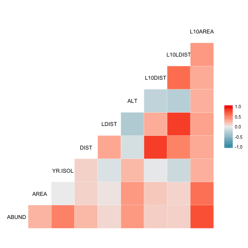
ggcorr(bird_abund[, 1:10], geom = "blank", label = TRUE, hjust = 0.75) +
  geom_point(size = 10, aes(color = coefficient > 0, alpha = abs(coefficient) > 0.5)) +
  scale_alpha_manual(values = c("TRUE" = 0.25, "FALSE" = 0)) +
  guides(color = FALSE, alpha = FALSE)
## Warning in ggcorr(bird_abund[, 1:10], geom = "blank", label = TRUE, hjust =
## 0.75): data in column(s) 'GRAZE' are not numeric and were ignored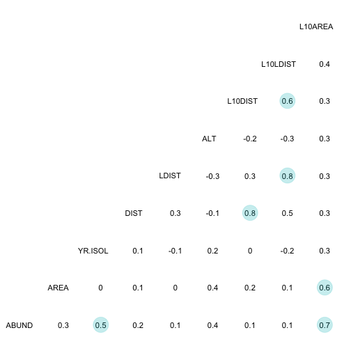
We run the regression similarly to the simple regression model.
bird_mod <- lm(ABUND ~ L10AREA + L10DIST + L10LDIST + GRAZE + ALT + YEAR_SINCE, data = bird_abund)

summary(bird_mod)
##
## Call:
## lm(formula = ABUND ~ L10AREA + L10DIST + L10LDIST + GRAZE + ALT +
## YEAR_SINCE, data = bird_abund)
##
## Residuals:
## Min 1Q Median 3Q Max
## -15.8992 -2.7245 -0.2772 2.7052 11.2811
##
## Coefficients:
## Estimate Std. Error t value Pr(>|t|)
## (Intercept) 11.29669 8.46090 1.335 0.1884
## L10AREA 6.83303 1.50330 4.545 0.0000397 ***
## L10DIST 0.33286 2.74778 0.121 0.9041
## L10LDIST 0.79765 2.13759 0.373 0.7107
## GRAZE2 0.52851 3.25221 0.163 0.8716
## GRAZE3 0.06601 2.95871 0.022 0.9823
## GRAZE4 -1.24877 3.19838 -0.390 0.6980
## GRAZE5 -12.47309 4.77827 -2.610 0.0122 *
## ALT 0.01070 0.02390 0.448 0.6565
## YEAR_SINCE 0.01277 0.05803 0.220 0.8267
## ---
## Signif. codes: 0 '***' 0.001 '**' 0.01 '*' 0.05 '.' 0.1 ' ' 1
##
## Residual standard error: 6.105 on 46 degrees of freedom
## Multiple R-squared: 0.7295, Adjusted R-squared: 0.6766
## F-statistic: 13.78 on 9 and 46 DF, p-value: 2.115e-10anova(bird_mod)## Analysis of Variance Table
##
## Response: ABUND
## Df Sum Sq Mean Sq F value Pr(>F)
## L10AREA 1 3471.0 3471.0 93.1303 1.247e-12 ***
## L10DIST 1 65.5 65.5 1.7568 0.1915648
## L10LDIST 1 136.5 136.5 3.6630 0.0618676 .
## GRAZE 4 938.6 234.6 6.2958 0.0003977 ***
## ALT 1 10.1 10.1 0.2718 0.6046450
## YEAR_SINCE 1 1.8 1.8 0.0485 0.8267495
## Residuals 46 1714.4 37.3
## ---
## Signif. codes: 0 '***' 0.001 '**' 0.01 '*' 0.05 '.' 0.1 ' ' 1And now take a look at the prediction with the residuals. First we want to use the augment() function from the broom package to create the predictions.
mod_pred <- augment(bird_mod)
glimpse(mod_pred)
## Observations: 56
## Variables: 14
## $ ABUND <dbl> 5.3, 2.0, 1.5, 17.1, 13.8, 14.1, 3.8, 2.2, 3.3, 3.0...
## $ L10AREA <dbl> -1.0000000, -0.3010300, -0.3010300, 0.0000000, 0.00...
## $ L10DIST <dbl> 1.591065, 2.369216, 2.017033, 1.819544, 2.390935, 2...
## $ L10LDIST <dbl> 1.591065, 2.369216, 2.492760, 1.819544, 2.390935, 2...
## $ GRAZE <fctr> 2, 5, 5, 3, 5, 3, 5, 5, 4, 5, 3, 5, 2, 1, 5, 5, 3,...
## $ ALT <int> 160, 60, 140, 160, 140, 130, 90, 60, 130, 130, 210,...
## $ YEAR_SINCE <dbl> 19, 67, 87, 21, 69, 22, 32, 67, 22, 87, 61, 97, 14,...
## $ .fitted <dbl> 8.7455613, 0.9429609, 2.0357546, 15.3999285, 3.9059...
## $ .se.fit <dbl> 3.248195, 2.317437, 2.166315, 2.065503, 2.074047, 2...
## $ .resid <dbl> -3.4455613, 1.0570391, -0.5357546, 1.7000715, 9.894...
## $ .hat <dbl> 0.2830886, 0.1440967, 0.1259162, 0.1144695, 0.11541...
## $ .sigma <dbl> 6.142511, 6.170043, 6.171802, 6.166515, 5.969861, 6...
## $ .cooksd <dbl> 0.0175448451, 0.0005896914, 0.0001269244, 0.0011320...
## $ .std.resid <dbl> -0.66657084, 0.18715342, -0.09386602, 0.29592694, 1...scatter_with_box(xvar=".fitted",yvar=".resid", xlim=c(0,45), ylim=c(-20,20), xlabel ="Predicted value", ylabel = "Residual", data=mod_pred)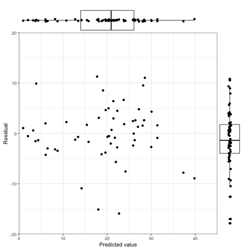
Predictions
There is an increased level of complication when u
Interactions
So far the models we have been working on have been additive. Often when researching biological situations, we might anticipate that there are interactions between the independent variables where the influence on our dependent variable is multiplicative.
Take for an example this model:
This assumes that the partial regression slope of \( Y \) on \( X_1 \) is independent of \( X_2 \) and vice-versa.
Consider this model:
The new term \( \beta_3 \) in this model represents the interactive effect of \( X_1 \) and \( X_2 \) on Y. It measures the dependence of the partial regression slope of Y against \( X_1 \) on the value of \( X_2 \) and the dependence of the partial regression slope of Y against \( X_2 \) on the value of \( X_1 \). These partial slopes are no longer independent.
To look at this, lets use the the parulo.csv data set in chapt06
paruelo <- read_csv("https://raw.githubusercontent.com/chrischizinski/SNR_R_Group/master/data/ExperimentalDesignData/chpt06/paruelo.csv")## Parsed with column specification:
## cols(
## C3 = col_double(),
## C4 = col_double(),
## MAP = col_integer(),
## MAT = col_double(),
## JJAMAP = col_double(),
## DJFMAP = col_double(),
## LONG = col_double(),
## LAT = col_double(),
## LC3 = col_double(),
## LC4 = col_double(),
## CLONG = col_double(),
## CLAT = col_double(),
## RESID1 = col_double(),
## PREDICT1 = col_double()
## )glimpse(paruelo)## Observations: 73
## Variables: 14
## $ C3 <dbl> 0.65, 0.65, 0.76, 0.75, 0.33, 0.03, 0.00, 0.02, 0.05,...
## $ C4 <dbl> 0.00, 0.00, 0.01, 0.18, 0.28, 0.83, 0.31, 0.87, 0.72,...
## $ MAP <int> 199, 469, 536, 476, 484, 623, 259, 969, 542, 421, 446...
## $ MAT <dbl> 12.4, 7.5, 7.2, 8.2, 4.8, 12.0, 14.5, 15.3, 13.9, 8.5...
## $ JJAMAP <dbl> 0.12, 0.24, 0.24, 0.35, 0.40, 0.40, 0.47, 0.30, 0.44,...
## $ DJFMAP <dbl> 0.45, 0.29, 0.20, 0.15, 0.14, 0.11, 0.17, 0.14, 0.13,...
## $ LONG <dbl> 119.55, 114.27, 110.78, 101.87, 102.82, 99.38, 106.75...
## $ LAT <dbl> 46.40, 47.32, 45.78, 43.95, 46.90, 38.87, 32.62, 36.9...
## $ LC3 <dbl> -0.124938737, -0.124938737, -0.065501549, -0.07058107...
## $ LC4 <dbl> -1.00000000, -1.00000000, -0.95860731, -0.55284197, -...
## $ CLONG <dbl> 13.149863, 7.869863, 4.379863, -4.530137, -3.580137, ...
## $ CLAT <dbl> 6.2957534, 7.2157534, 5.6757534, 3.8457534, 6.7957534...
## $ RESID1 <dbl> -0.029229334, -0.028808495, 0.168066337, 0.323799098,...
## $ PREDICT1 <dbl> -0.09570940, -0.09613024, -0.23356789, -0.39438017, -...Lets fit a couple of models of the abundance of the C3 grasses with Lattitude, Longitude, and then all variables with an interaction.
mod1 <- lm(C3 ~ LAT, data = paruelo)
mod2 <- lm(C3 ~ LONG, data = paruelo)
mod3 <- lm(C3 ~ LAT+LONG, data = paruelo)
mod4 <- lm(C3 ~ LAT*LONG, data = paruelo)

summary(mod1)
##
## Call:
## lm(formula = C3 ~ LAT, data = paruelo)
##
## Residuals:
## Min 1Q Median 3Q Max
## -0.40210 -0.15689 -0.00521 0.14165 0.40301
##
## Coefficients:
## Estimate Std. Error t value Pr(>|t|)
## (Intercept) -1.045735 0.176115 -5.938 9.70e-08 ***
## LAT 0.032842 0.004354 7.543 1.17e-10 ***
## ---
## Signif. codes: 0 '***' 0.001 '**' 0.01 '*' 0.05 '.' 0.1 ' ' 1
##
## Residual standard error: 0.1959 on 71 degrees of freedom
## Multiple R-squared: 0.4449, Adjusted R-squared: 0.437
## F-statistic: 56.89 on 1 and 71 DF, p-value: 1.175e-10summary(mod2)##
## Call:
## lm(formula = C3 ~ LONG, data = paruelo)
##
## Residuals:
## Min 1Q Median 3Q Max
## -0.29063 -0.21921 -0.06637 0.20256 0.61641
##
## Coefficients:
## Estimate Std. Error t value Pr(>|t|)
## (Intercept) 0.092073 0.512844 0.18 0.858
## LONG 0.001685 0.004811 0.35 0.727
##
## Residual standard error: 0.2627 on 71 degrees of freedom
## Multiple R-squared: 0.001725, Adjusted R-squared: -0.01234
## F-statistic: 0.1227 on 1 and 71 DF, p-value: 0.7272summary(mod3)##
## Call:
## lm(formula = C3 ~ LAT + LONG, data = paruelo)
##
## Residuals:
## Min 1Q Median 3Q Max
## -0.41150 -0.15666 -0.00401 0.14823 0.40703
##
## Coefficients:
## Estimate Std. Error t value Pr(>|t|)
## (Intercept) -0.9504806 0.4094130 -2.322 0.0232 *
## LAT 0.0329518 0.0044035 7.483 1.63e-10 ***
## LONG -0.0009366 0.0036287 -0.258 0.7971
## ---
## Signif. codes: 0 '***' 0.001 '**' 0.01 '*' 0.05 '.' 0.1 ' ' 1
##
## Residual standard error: 0.1972 on 70 degrees of freedom
## Multiple R-squared: 0.4454, Adjusted R-squared: 0.4295
## F-statistic: 28.11 on 2 and 70 DF, p-value: 1.096e-09summary(mod4)##
## Call:
## lm(formula = C3 ~ LAT * LONG, data = paruelo)
##
## Residuals:
## Min 1Q Median 3Q Max
## -0.39563 -0.14722 -0.01491 0.11837 0.40268
##
## Coefficients:
## Estimate Std. Error t value Pr(>|t|)
## (Intercept) 6.7518079 2.9399294 2.297 0.0247 *
## LAT -0.1618176 0.0737967 -2.193 0.0317 *
## LONG -0.0752581 0.0283285 -2.657 0.0098 **
## LAT:LONG 0.0018773 0.0007101 2.644 0.0101 *
## ---
## Signif. codes: 0 '***' 0.001 '**' 0.01 '*' 0.05 '.' 0.1 ' ' 1
##
## Residual standard error: 0.1893 on 69 degrees of freedom
## Multiple R-squared: 0.4964, Adjusted R-squared: 0.4745
## F-statistic: 22.67 on 3 and 69 DF, p-value: 2.525e-10Interpretation
The estimate of \( \beta_{1} \) is the regression slope of Y on \( X_1 \) when \( X_2 \) is constant. If there is an interaction (i.e., \( \beta_{3} \) does not equal zero), the slope will change for values of \( X_2 \); if there is not an interaction \( \beta_{3} \) = 0), then this slope will be constant for all levels of \(X_2\). Thus, when there is a significant interaction, we care little about the main effects in the model.
range(paruelo$LAT)## [1] 29.00 52.13range(paruelo$LONG)## [1] 93.20 119.55newdata <- expand.grid(LAT = seq(min(paruelo$LAT), max(paruelo$LAT), by = 1),
LONG = range(paruelo$LONG))
mod_pred1 <- augment(mod3, newdata = newdata)
mod_pred2 <- augment(mod4, newdata = newdata)ggplot(data = mod_pred1) +
geom_line(aes(x = LAT, y= .fitted, colour=as.factor(LONG)), size = 1) +
labs(x = "Lattitude", y = "C3 Grass abundance", title ="No interaction") +
theme_bw()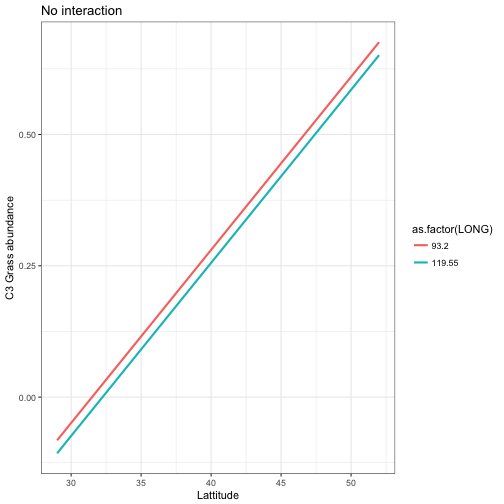
p1<-ggplot(data = mod_pred2) +
  geom_line(aes(x = LAT, y= .fitted, colour=as.factor(LONG)), size = 1) +
  labs(x = "Lattitude", y = "C3 Grass abundance", title ="With interaction") +
  theme_bw()

p1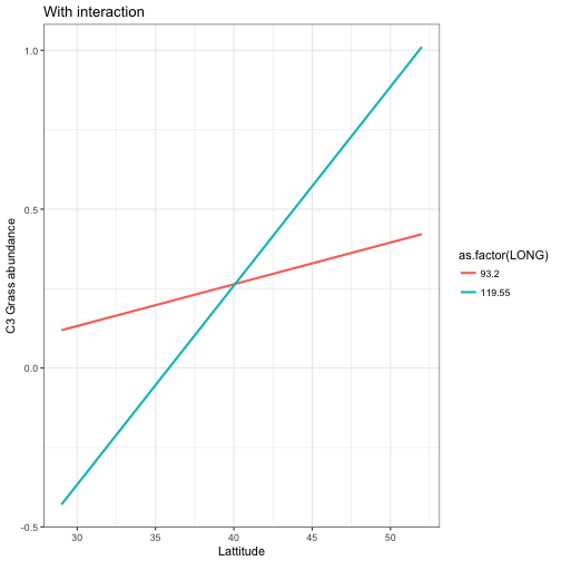
Centering
One issue with including interactions, is that \(X_1\) and \(X_2\) are highly correlated with \(X_1* X_2\).
As an example lets look at LAT and LONG
paruelo$LATxLONG <- paruelo$LAT * paruelo$LONG


ggcorr(paruelo[, c(1,7,8,15)], geom = "blank", label = TRUE, hjust = 0.75) +
  geom_point(size = 10, aes(color = coefficient > 0, alpha = abs(coefficient) > 0.5)) +
  scale_alpha_manual(values = c("TRUE" = 0.25, "FALSE" = 0)) +
  guides(color = FALSE, alpha = FALSE)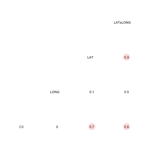
Remember that with highly correlated variables are all the computational issues as well as inflated variances of the coefficients. One way to get around the high degree of multicollinearity is centering.
When we have an interaction in the model, the estimated slope for Y on \(X_1\) when \(X_2\) is zero is not very informative because zero is not usually within the range of our observations for any of the predictor variables. Remember the ranges of our LAT and LONG variables.
However, if the predictors are centered, then the estimate of \( \beta_1 \) is now the regression slope of Y on \( X_1 \) for the mean of \( X_1 \).
paruelo$CLAT <- as.numeric(scale(paruelo$LAT, center = TRUE, scale = FALSE))
paruelo$CLONG <- as.numeric(scale(paruelo$LONG, center = TRUE, scale = FALSE))

mod5 <- lm(C3 ~ CLAT*CLONG, data = paruelo)
summary(mod5)
##
## Call:
## lm(formula = C3 ~ CLAT * CLONG, data = paruelo)
##
## Residuals:
## Min 1Q Median 3Q Max
## -0.39563 -0.14722 -0.01491 0.11837 0.40268
##
## Coefficients:
## Estimate Std. Error t value Pr(>|t|)
## (Intercept) 0.26526887 0.02227470 11.909 < 2e-16 ***
## CLAT 0.03792436 0.00462612 8.198 8.69e-12 ***
## CLONG 0.00002852 0.00350182 0.008 0.9935
## CLAT:CLONG 0.00187727 0.00071012 2.644 0.0101 *
## ---
## Signif. codes: 0 '***' 0.001 '**' 0.01 '*' 0.05 '.' 0.1 ' ' 1
##
## Residual standard error: 0.1893 on 69 degrees of freedom
## Multiple R-squared: 0.4964, Adjusted R-squared: 0.4745
## F-statistic: 22.67 on 3 and 69 DF, p-value: 2.525e-10range(paruelo$CLAT)## [1] -11.10425 12.02575range(paruelo$CLONG)## [1] -13.20014 13.14986newdata <- expand.grid(CLAT = seq(min(paruelo$CLAT), max(paruelo$CLAT), by = 1),
CLONG = range(paruelo$CLONG))
mod_pred3 <- augment(mod5, newdata = newdata)p2<-ggplot(data = mod_pred3) +
geom_line(aes(x = CLAT, y= .fitted, colour=as.factor(CLONG)), size = 1) +
labs(x = "Lattitude", y = "C3 Grass abundance", title ="Centered") +
theme_bw()
grid.arrange(p1,p2, ncol=2)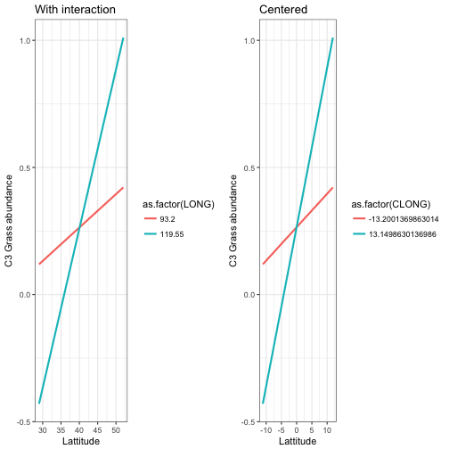
What can be some issues with centering?
Selecting against competing models
library(AICcmodavg)

cand.models <- list()

cand.models[[1]] <- lm(C3~ LAT, data = paruelo)
cand.models[[2]] <- lm(C3~ LONG, data = paruelo)
cand.models[[3]] <- lm(C3~ LAT+LONG, data = paruelo)
cand.models[[4]] <- lm(C3~ LAT*LONG, data = paruelo)

mod.names <-c("Lat only","Long only","Lat Long additive","Lat Long interaction")

aictab(cand.set = cand.models, modnames = mod.names)
##
## Model selection based on AICc:
##
## K AICc Delta_AICc AICcWt Cum.Wt LL
## Lat Long interaction 5 -29.07 0.00 0.73 0.73 19.98
## Lat only 3 -26.50 2.56 0.20 0.93 16.42
## Lat Long additive 4 -24.33 4.74 0.07 1.00 16.46
## Long only 3 16.34 45.40 0.00 1.00 -4.99