The RMarkdown file for this lesson can be found here.
This lesson will follow Chapter 5 in Quinn and Keough (2002).
Load the packages we will be using in this lesson
library(MASS)
library(car)
library(RCurl)
library(mgcv)
library(tidyverse)
library(broom)
library(Rfit)
library(mgcv)
library(gtable)
library(lmodel2)
Linear regression analysis
Statistical models that assume a linear relationship between a single, continuous (usually) predictor value are simple linear regression models.
These models have three primary purposes:
- describe a linear relationship between \( Y \) and \( X \)
- determine the amount of variation (explained) in \( Y \) with \( X \) and the amount of variation unexplained
- predict values of \( Y \) from \( X \)
Simple bivariate linear regression
Linear model for regression
Consider you have a set of observations (\( i = 1 :n \) ), where the each observation was chosen based on its \( X \) value and its \( Y \) value for each observation is sampled from a population of possible \( Y \) values.
This model can be represented as:
- \( y_i \) is the value of \( Y \) for the ith observation when the predictor \( X = x_i \)
- \( \beta_0 \) is the population intercept (i.e., mean value of the probability distribution) when \( x_i = 0\)
- \( \beta_1 \) is the population slope and measures the change in \( Y \) with a change in \( X \)
- \( \epsilon_i \) is the random or unexplained error associated with the ith observation
In this model, the response variable \( Y \) is a random variable and \( X \) represents fixed values choed by the researcher. Thus repeated sampling, you would have the same values of \( X \) while \( Y \) would vary.
Estimating model parameters
The main goal in regression analysis is estimating \( \beta_0 \), \( \beta_1 \), and \( \sigma_\epsilon^2 \).
We discussed solving for \( \beta_0 \) and \( \beta_1 \) using OLS in an earlier lesson
Regression slope
The most informative of the parameters in a regression equation is \( \beta_{1} \), because this describes the relationship between \( Y \) and \( X \).
Intercept
The OLS regression line must pass through \( \bar{x} \) and \( \bar{y} \). We can then estimate \( \beta_{0} \) by substituting in \( \beta_{1} \), \( \bar{x} \) and \( \bar{y} \).
Often the intercept does not contain a lot of usable information because rarely do we have situations where \( X = 0 \).
Lets begin to explore this with the coarse woody debris data in lakes. christ data in Chap 5 on github.
cwd_data <- read_csv(getURL('https://raw.githubusercontent.com/chrischizinski/SNR_R_Group/master/data/ExperimentalDesignData/chpt05/christ.csv'))

glimpse(cwd_data)
## Observations: 16
## Variables: 17
## $ LAKE <chr> "Bay", "Bergner", "Crampton", "Long", "Roach", "Tende...
## $ AREA <int> 69, 9, 24, 8, 20, 175, 254, 22, 240, 85, 12, 25, 58, ...
## $ CABIN <dbl> 0.0, 0.0, 0.0, 0.0, 0.0, 0.6, 1.9, 3.6, 4.1, 4.8, 6.0...
## $ RIP.DENS <int> 1270, 1210, 1800, 1875, 1300, 2150, 1330, 964, 961, 1...
## $ RIP.BASA <int> 53, 37, 37, 27, 43, 75, 86, 35, 33, 28, 47, 30, 31, 3...
## $ CWD.DENS <int> 442, 338, 965, 833, 613, 637, 298, 203, 48, 278, 316,...
## $ CWD.BASA <int> 121, 41, 183, 130, 127, 134, 65, 52, 12, 46, 54, 97, ...
## $ L10CABIN <dbl> 0.0000000, 0.0000000, 0.0000000, 0.0000000, 0.0000000...
## $ LCWD.BAS <dbl> 2.082785, 1.612784, 2.262451, 2.113943, 2.103804, 2.1...
## $ RESID1 <dbl> 51.393669, -21.675367, 52.170151, -9.493554, 53.92818...
## $ PREDICT1 <dbl> 69.60633, 62.67537, 130.82985, 139.49355, 73.07181, 1...
## $ RESID2 <dbl> 20.600685, -59.399315, 82.600685, 29.600685, 26.60068...
## $ PREDICT2 <dbl> 100.399315, 100.399315, 100.399315, 100.399315, 100.3...
## $ RESID3 <dbl> -0.968746, -80.968746, 61.031254, 8.031254, 5.031254,...
## $ PREDICT3 <dbl> 121.968746, 121.968746, 121.968746, 121.968746, 121.9...
## $ RESID4 <dbl> -0.11210186, -0.58210286, 0.06756414, -0.08094386, -0...
## $ PREDICT4 <dbl> 2.1948869, 2.1948869, 2.1948869, 2.1948869, 2.1948869...ggplot(data = cwd_data) +
geom_point(aes(x = RIP.DENS, y = CWD.DENS), size = 2) +
labs(x = "Riparian tree density", y ="Coarse woody debris density") +
theme_bw()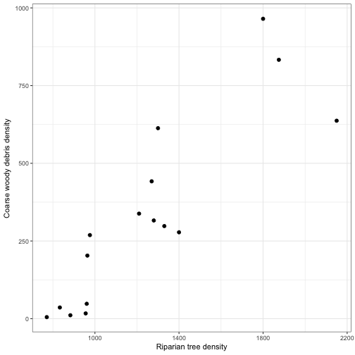
`lm()’ is the function in R to conduct simple linear regression.
mod_cwd <- lm(CWD.DENS ~  RIP.DENS, data = cwd_data)

mod_cwd # displays the coefficients
##
## Call:
## lm(formula = CWD.DENS ~ RIP.DENS, data = cwd_data)
##
## Coefficients:
## (Intercept) RIP.DENS
## -482.0245 0.6524summary(mod_cwd) # displays a bunch more information##
## Call:
## lm(formula = CWD.DENS ~ RIP.DENS, data = cwd_data)
##
## Residuals:
## Min 1Q Median 3Q Max
## -283.65 -89.99 -20.71 92.69 272.69
##
## Coefficients:
## Estimate Std. Error t value Pr(>|t|)
## (Intercept) -482.0245 126.5724 -3.808 0.00192 **
## RIP.DENS 0.6524 0.0969 6.733 0.00000958 ***
## ---
## Signif. codes: 0 '***' 0.001 '**' 0.01 '*' 0.05 '.' 0.1 ' ' 1
##
## Residual standard error: 150.2 on 14 degrees of freedom
## Multiple R-squared: 0.764, Adjusted R-squared: 0.7472
## F-statistic: 45.33 on 1 and 14 DF, p-value: 0.000009581There is a lot of information stored in our object mod_cwd.
names(mod_cwd)## [1] "coefficients" "residuals" "effects" "rank"
## [5] "fitted.values" "assign" "qr" "df.residual"
## [9] "xlevels" "call" "terms" "model"We can call on these directly from our mod_cwd or use several ‘helper’ functions.
# Coefficients
mod_cwd$coefficients
## (Intercept) RIP.DENS
## -482.0245271 0.6524071#or
coef(mod_cwd)## (Intercept) RIP.DENS
## -482.0245271 0.6524071# Residuals
mod_cwd$residuals[1:10] # display the first 10 residuals## 1 2 3 4 5 6
## 95.46757 30.61199 272.69183 91.76130 246.89535 -283.65064
## 7 8 9 10
## -87.67686 56.10412 -96.93865 -153.34535#or
resid(mod_cwd)[1:10]## 1 2 3 4 5 6
## 95.46757 30.61199 272.69183 91.76130 246.89535 -283.65064
## 7 8 9 10
## -87.67686 56.10412 -96.93865 -153.34535mod_cwd$model## CWD.DENS RIP.DENS
## 1 442 1270
## 2 338 1210
## 3 965 1800
## 4 833 1875
## 5 613 1300
## 6 637 2150
## 7 298 1330
## 8 203 964
## 9 48 961
## 10 278 1400
## 11 316 1280
## 12 269 976
## 13 5 771
## 14 36 833
## 15 11 883
## 16 17 956The broom package makes inspection of the models a bit easier (although they are not too difficult) in base R. The biggest plus for broom, is that the outputs of the models are returned in a tidy format.
# tidy will give you a data.frame representation
tidy(mod_cwd)
## term estimate std.error statistic p.value
## 1 (Intercept) -482.0245271 126.57242447 -3.808290 0.001919139303
## 2 RIP.DENS 0.6524071 0.09689906 6.732852 0.000009581278# augment will give fitted values and residuals for each of the original points in the regression
head(augment(mod_cwd))## CWD.DENS RIP.DENS .fitted .se.fit .resid .hat .sigma
## 1 442 1270 346.5324 37.60939 95.46757 0.06271192 153.4340
## 2 338 1210 307.3880 37.72064 30.61199 0.06308346 155.6054
## 3 965 1800 692.3082 65.39508 272.69183 0.18960407 131.2693
## 4 833 1875 741.2387 71.46726 91.76130 0.22644969 153.1426
## 5 613 1300 366.1046 37.88968 246.89535 0.06365013 138.8604
## 6 637 2150 920.6506 95.17612 -283.65064 0.40161828 118.0974
## .cooksd .std.resid
## 1 0.014422585 0.6565957
## 2 0.001492878 0.2105813
## 3 0.475910054 2.0169830
## 4 0.070638454 0.6946947
## 5 0.098101659 1.6989187
## 6 2.000561396 -2.4415935#glance will let you see the statistics associated with the model
glance(mod_cwd)## r.squared adj.r.squared sigma statistic p.value df logLik
## 1 0.7640368 0.7471823 150.1832 45.3313 0.000009581278 2 -101.8245
## AIC BIC deviance df.residual
## 1 209.6489 211.9667 315769.8 14Confidence intervals
Confidence intervals for \( \beta_{1} \) are calculated in the usual manner when we know the standard error of a statistic and use the t distribution.
This can be represented as a confidence band (e.g. 95%) for the regression line. The 95% confidence band is a band that will contain the true population regression line 95% of the time.
We can display our confidence intervals using geom_smooth in ggplot.
ggplot(data = cwd_data) +
  geom_point(aes(x = RIP.DENS, y = CWD.DENS), size = 2) +
  geom_smooth(aes(x = RIP.DENS, y = CWD.DENS), method = 'lm', alpha = 0.35) +
  labs(x = "Riparian tree density", y ="Coarse woody debris density", title = "Linear model fit") +
  theme_bw()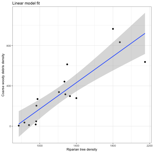
We can also use geom_smooth to explore other non-linear relationships between \( X \) and \( Y \).
ggplot(data = cwd_data) +
  geom_point(aes(x = RIP.DENS, y = CWD.DENS), size = 2) +
  geom_smooth(aes(x = RIP.DENS, y = CWD.DENS), method = 'loess', alpha = 0.35) +
  labs(x = "Riparian tree density", y ="Coarse woody debris density", title = "Loess fit") +
  theme_bw()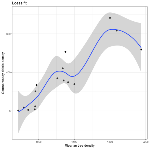
# or via a GAM

ggplot(data = cwd_data) +
  geom_point(aes(x = RIP.DENS, y = CWD.DENS), size = 2) +
  geom_smooth(aes(x = RIP.DENS, y = CWD.DENS), method = 'gam', alpha = 0.35) +
  labs(x = "Riparian tree density", y ="Coarse woody debris density", title = "GAM fit") +
  theme_bw()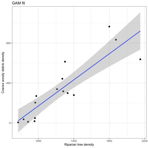
While using geom_smooth makes nice visuals, I think you have a lot more flexibility when you build your own predictions. The predict() function is one of my favorite functions in R.
Predicted values
Prediction from the OLS regression equation is straightforward by substituting an X-value into the regression equation and calculating the predicted Y-value. Do not predict from X-values outside the range of your data.
If we run the predict() with just the model, we get results the same as in the fitted.values.
pred_values <- predict(mod_cwd)
head(pred_values)
## 1 2 3 4 5 6
## 346.5324 307.3880 692.3082 741.2387 366.1046 920.6506# pulling out the values using augment
head(augment(mod_cwd)$.fitted)## [1] 346.5324 307.3880 692.3082 741.2387 366.1046 920.6506It helps to bind, your predictions (and the standard error) with those from your original data. NOTE: that augment already does this for you.
fitted_vals <- cbind(cwd_data[,c("RIP.DENS","CWD.DENS")],predict(mod_cwd, se.fit = TRUE))

ggplot(data = fitted_vals) +
  geom_point(aes(x = RIP.DENS, y = CWD.DENS), size = 2) +
  geom_ribbon(aes(x = RIP.DENS, ymax = fit + 1.96*se.fit, ymin = fit - 1.96*se.fit), fill="#0E3386", alpha = 0.5) +
  geom_line(aes(x = RIP.DENS, y = fit), color = "#D12325", size = 1, linetype = "dashed") +
  coord_cartesian(ylim = c(0, 1000), expand = FALSE)  +
  scale_y_continuous(breaks = seq(0,1000, by = 250)) +
  labs(x = "Riparian tree density", y ="Coarse woody debris density") +
  theme_bw()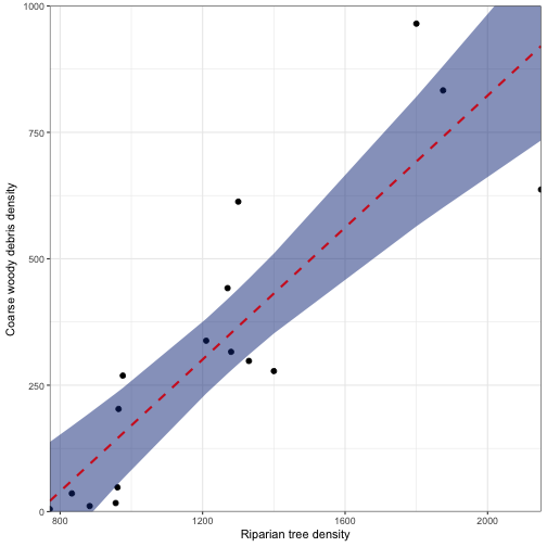
While these values are helpful in displaying the basic model fit, there are often times (especially when doing multiple linear regression) when you want to look at predictions based off specific values. We can do this by using the newdata in predict(). NOTE that the column header names need to reflect the independent values in your model.
nd <- data.frame(RIP.DENS = 800:2100)

fitted_vals <- cbind(nd,predict(mod_cwd,newdata = nd, se.fit = TRUE))

head(fitted_vals)
## RIP.DENS fit se.fit df residual.scale
## 1 800 39.90112 57.35375 14 150.1832
## 2 801 40.55352 57.28054 14 150.1832
## 3 802 41.20593 57.20739 14 150.1832
## 4 803 41.85834 57.13432 14 150.1832
## 5 804 42.51075 57.06132 14 150.1832
## 6 805 43.16315 56.98838 14 150.1832ggplot(data = fitted_vals) +
geom_ribbon(aes(x = RIP.DENS, ymax = fit + 1.96*se.fit, ymin = fit - 1.96*se.fit), fill="#ED174C", alpha = 0.5) +
geom_line(aes(x = RIP.DENS, y = fit), color = "#002B5C", size = 1, linetype = "dashed") +
coord_cartesian(ylim = c(0, 1000), expand = FALSE) +
scale_y_continuous(breaks = seq(0,1000, by = 250)) +
labs(x = "Riparian tree density", y ="Coarse woody debris density") +
theme_bw()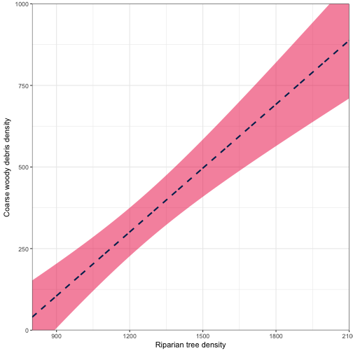
Residuals
This difference between each observed \( y_{i} \) and each predicted \( \hat{y_i} \) is called a residual \( e_{i} \):
fitted_vals <- cbind(cwd_data[,c("RIP.DENS","CWD.DENS")],predict(mod_cwd, se.fit = TRUE))

ggplot(data = fitted_vals) +
    geom_segment(aes(x = RIP.DENS, xend = RIP.DENS,  y = CWD.DENS, yend = fit), linetype = 'dotted', alpha = 0.5) +
  geom_point(aes(x = RIP.DENS, y = CWD.DENS), size = 1, colour ="black") +
  geom_point(aes(x = RIP.DENS, y = fit), size = 1, colour ="red") +
  labs(x = "Riparian tree density", y ="Coarse woody debris density") +
  theme_bw()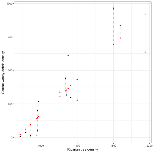
Analysis of variance
In biological sciences we often want to partition the total variation in \( Y \) in part to \( X \) and the other part to the unexplained variation. The partitioned variance is often presented as an analysis of variance (ANOVA) table.
- Total variation in \( Y \) is the sum of squared deviations of each observation from the sample mean
- \( SS_{total} \) has n-1 df and can be partitioned into two additive components
-
Variation in \( Y \) explained by \( X \) (difference between \( \hat{y_i} \) and \( \bar{y} \). The number of degrees of freedom associated with a linear model is usually the number of parameters minus one.
-
Variation in \( Y \) not explained by \( X \) (difference between each observed Y-value and \( \hat{y_i} \). Residual (or error) variation. The \( df_{residual} \) is n-2, because we have already estimated \( \beta_0 \) and \( \beta_1 \) to determine the \( \hat{y_i} \).
- The SS and df are additive
ggplot(data = fitted_vals) +
    geom_segment(data = fitted_vals[fitted_vals$RIP.DENS==1400,],
                 aes(x = RIP.DENS, xend = RIP.DENS,  y = CWD.DENS, yend = fit), linetype = 'dotted') +
  geom_segment(data = fitted_vals[fitted_vals$RIP.DENS==1800,],
                 aes(x = RIP.DENS, xend = RIP.DENS,  y = mean(fitted_vals$CWD.DENS), yend = fit), linetype = 'dotted') +
  geom_point(aes(x = RIP.DENS, y = CWD.DENS), size = 1, colour ="black") +
  geom_point(aes(x = RIP.DENS, y = fit), size = 1, colour ="red") +
  labs(x = "Riparian tree density", y ="Coarse woody debris density") +
  annotate("text", x = 1800, y = mean(fitted_vals$CWD.DENS), label = ' hat(y)[1800]~-~bar(y)', parse =TRUE) +
  annotate("text", x = 1400, y = fitted_vals$CWD.DENS[fitted_vals$RIP.DENS==1400], label = ' hat(y)[1400]~-~Y[1400]', parse =TRUE) +
  theme_bw()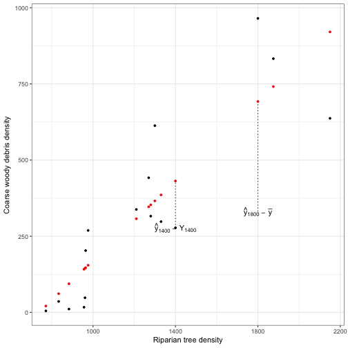
-
The \( SS_{total} \) increases with sample size. The Mean SS is a measure of variability that does not depend on sample size. MS is calculated by dividing SS by their df and thus, are not additive.
-
The \( MS_{Residual} \) estimates the common variance of the error terms \( e_{i} \), and therefore of the Y-values at each \( x_i \). NOTE a key assumption is homogeneity of variances.
We can calculate the ANOVA table from our linear model in R by using the anova() statment.
tidy(anova(mod_cwd))## term df sumsq meansq statistic p.value
## 1 RIP.DENS 1 1022446.7 1022446.67 45.3313 0.000009581278
## 2 Residuals 14 315769.8 22554.98 NA NAVariance explaned ( \(r^2\) or \( R^2 \))
-
descriptive measure of association between Y and X (also termed coefficient of variation). the proportion of the total variation in Y that is explained by its linear relationship with X.
-
\( 1 = \frac{SS_{residual}}{SS_{total}} \)
Scatterplot with marginal boxplots
## Create the base scatterplot

p1 <- ggplot(data = cwd_data) +
   geom_point(aes(x = RIP.DENS, y = CWD.DENS)) +
   scale_x_continuous(expand = c(0, 0)) +
   scale_y_continuous(expand = c(0, 0)) +
   coord_cartesian(xlim = c(700,2300), ylim = c(0,1000)) +
   theme_bw() +
   theme(plot.margin = unit(c(0.2, 0.2, 0.5, 0.5), "lines"))

# horizontal marginal boxplots

p2 <- ggplot(data = cwd_data) +
   geom_boxplot(aes(x = factor(1),y = RIP.DENS), outlier.colour = "red") +
   geom_jitter(aes(x = factor(1),y = RIP.DENS),position = position_jitter(width = 0.05)) +
   scale_y_continuous(expand = c(0, 0))  +
   coord_flip(ylim = c(700,2300)) +
   theme_void() +
   theme(axis.text = element_blank(),
         axis.title = element_blank(),
         axis.ticks = element_blank(),
         plot.margin = unit(c(1, 0.2, -0.5, 0.5), "lines"))

# vertical marginal boxplots

p3 <- ggplot(data = cwd_data) +
   geom_boxplot(aes(x = factor(1),y = CWD.DENS), outlier.colour = "red") +
   geom_jitter(aes(x = factor(1),y = CWD.DENS),position = position_jitter(width = 0.05)) +
   scale_y_continuous(expand = c(0, 0)) +
  coord_cartesian( ylim = c(0,1000)) +
  theme_void() +
   theme(axis.text = element_blank(),
         axis.title = element_blank(),
         axis.ticks = element_blank(),
         plot.margin = unit(c(0.2, 1, 0.5, -0.5), "lines"))
gt1 <- ggplot_gtable(ggplot_build(p1))
gt2 <- ggplot_gtable(ggplot_build(p2))
gt3 <- ggplot_gtable(ggplot_build(p3))# Get maximum widths and heights
maxWidth <- unit.pmax(gt1$widths[2:3], gt2$widths[2:3])
maxHeight <- unit.pmax(gt1$heights[4:5], gt3$heights[4:5])
# Set the maximums in the gtables for gt1, gt2 and gt3
gt1$widths[2:3] <- as.list(maxWidth)
gt2$widths[2:3] <- as.list(maxWidth)
gt1$heights[4:5] <- as.list(maxHeight)
gt3$heights[4:5] <- as.list(maxHeight)# Create a new gtable
gt <- gtable(widths = unit(c(7, 1), "null"), height = unit(c(1, 7), "null"))
# Insert gt1, gt2 and gt3 into the new gtable
gt <- gtable_add_grob(gt, gt1, 2, 1)
gt <- gtable_add_grob(gt, gt2, 1, 1)
gt <- gtable_add_grob(gt, gt3, 2, 2)
# And render the plot
grid.newpage()
grid.draw(gt)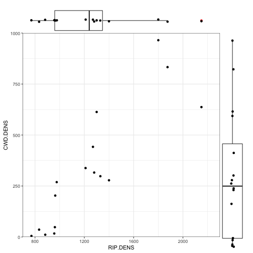
# grid.rect(x = 0.5, y = 0.5, height = 0.995, width = 0.995, default.units = "npc",
#     gp = gpar(col = "black", fill = NA, lwd = 1))
Assumptions of a regression model
- Normality (except GLMs)
- Homogeneity of variance
- Independence
- Fixed X
Regression diagnostics
- A proper interpretation of a linear regression analysis should also include checks of how well the model fits the observed data
- Is a straight line appropriate?
- Influence of outliers?
- See-saw, balanced on the mean of X
Leverage
-
Leverage is a measure of how extreme an observation is for the \(X \)-variable
-
Generally concerned when a value is 2 or 3 times greater than the mean value
fitted_vals2 <- cbind(cwd_data[,c("RIP.DENS","CWD.DENS")],predict(mod_cwd, se.fit = TRUE))

mod_hat<-hatvalues(mod_cwd)
mean_hat <- mean(mod_hat)

fitted_vals2$resid.out <- 0

fitted_vals2$resid.out[which(mod_hat > 2*mean_hat)] <- 1

fitted_vals2$resid.out <- as.factor(fitted_vals2$resid.out )

ggplot(data = fitted_vals2)  +
  geom_point(aes(x = RIP.DENS, y = CWD.DENS, colour = resid.out), size = 2) +
  geom_line(aes(x = RIP.DENS, y = fit), color = "#002B5C", size = 1, linetype = "dashed") +
  coord_cartesian(ylim = c(0, 1000), xlim = c(750, 2200), expand = FALSE)  +
  scale_y_continuous(breaks = seq(0,1000, by = 250)) +
  labs(x = "Riparian tree density", y ="Coarse woody debris density") +
  scale_colour_manual(values = c("0" = "red", "1" = "blue")) +
  theme_bw() +
  theme(legend.position = c(0.90, 0.25))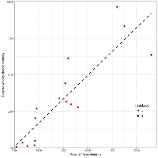
Residuals
-
Residuals are an important way of checking regression assumptions
-
Studentized residuals do have constant variance so different studentized residuals can be compared
std_res <- studres(mod_cwd)

fitted_vals2$resid.std <- std_res

ggplot(data = fitted_vals2)  +
  geom_point(aes(x = RIP.DENS, y = resid.std), size = 2) +
  coord_cartesian(ylim = c(-4, 4), xlim = c(750, 2200), expand = FALSE)  +
  scale_y_continuous(breaks = seq(-4,4, by = 1)) +
  labs(x = "Riparian tree density", y ="Coarse woody debris density") +
  scale_colour_manual(values = c("0" = "red", "1" = "blue")) +
  theme_bw()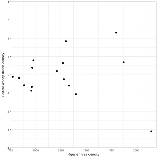
#outlier.test in car package
outlierTest(mod_cwd)
##
## No Studentized residuals with Bonferonni p < 0.05
## Largest |rstudent|:
## rstudent unadjusted p-value Bonferonni p
## 6 -3.104947 0.0083667 0.13387Influence
-
Cook’s distance statistic, \( D_i \), is the measure of the influence each observation has on the fitted regression line and the estimates of the regression parameters.
-
A large \( D_i \) indicates that removal of that observation would change the estimates of the regression parameters considerably
fitted_vals3<-augment(mod_cwd)

ggplot(data = fitted_vals3)  +
  geom_point(aes(x = RIP.DENS, y = CWD.DENS, colour = .cooksd ), size = 2) +
  coord_cartesian(ylim = c(0, 1000), xlim = c(750, 2200), expand = FALSE)  +
  scale_y_continuous(breaks = seq(0,1000, by = 250)) +
  labs(x = "Riparian tree density", y ="Coarse woody debris density") +
  scale_colour_continuous(low = "black", high = "red") +
  theme_bw()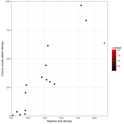
Weighted least squares
- Responses are averages with known sample sizes
- Responses are estimates and SEs are available
- \( w_i = \frac{1}{se(Y_i)^2} \)
- Variance is proportional to X
- \( w_i = \frac{1}{X_i} \) or \( w_i = \frac{1}{X_i^2} \)
set.seed(12345)

x = rnorm(100,0,3)
y = 3-2*x + rnorm(100,0,sapply(x,function(x){1+0.5*x^2}))

fake_data1 <- data.frame(x = x, y = y)

mod_1 <- lm(y ~ x, data = fake_data1)
summary(mod_1)
##
## Call:
## lm(formula = y ~ x, data = fake_data1)
##
## Residuals:
## Min 1Q Median 3Q Max
## -29.1365 -1.9392 0.4543 3.2609 27.8710
##
## Coefficients:
## Estimate Std. Error t value Pr(>|t|)
## (Intercept) 2.5684 0.8601 2.986 0.00357 **
## x -1.3402 0.2524 -5.310 0.000000685 ***
## ---
## Signif. codes: 0 '***' 0.001 '**' 0.01 '*' 0.05 '.' 0.1 ' ' 1
##
## Residual standard error: 8.398 on 98 degrees of freedom
## Multiple R-squared: 0.2234, Adjusted R-squared: 0.2155
## F-statistic: 28.19 on 1 and 98 DF, p-value: 0.000000685fake_pred<-cbind(fake_data1, predict(mod_1, se.fit = TRUE))
ggplot(data = fake_pred) +
geom_point(aes(x = x, y = y), size = 2, colour = "red") +
geom_line(aes(x = x, y = fit), linetype = 'dashed') +
theme_bw()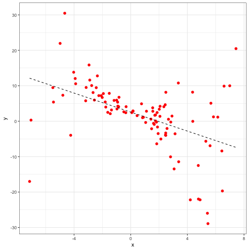
mod_2 <- lm(y ~ x, weights= 1/(x^2), data = fake_data1)
summary(mod_2)
##
## Call:
## lm(formula = y ~ x, data = fake_data1, weights = 1/(x^2))
##
## Weighted Residuals:
## Min 1Q Median 3Q Max
## -4.4230 -1.0989 0.1181 1.4912 4.4567
##
## Coefficients:
## Estimate Std. Error t value Pr(>|t|)
## (Intercept) 2.7659 0.1213 22.794 < 2e-16 ***
## x -1.6554 0.2092 -7.911 3.92e-12 ***
## ---
## Signif. codes: 0 '***' 0.001 '**' 0.01 '*' 0.05 '.' 0.1 ' ' 1
##
## Residual standard error: 2.07 on 98 degrees of freedom
## Multiple R-squared: 0.3898, Adjusted R-squared: 0.3835
## F-statistic: 62.59 on 1 and 98 DF, p-value: 3.918e-12summary(mod_1)##
## Call:
## lm(formula = y ~ x, data = fake_data1)
##
## Residuals:
## Min 1Q Median 3Q Max
## -29.1365 -1.9392 0.4543 3.2609 27.8710
##
## Coefficients:
## Estimate Std. Error t value Pr(>|t|)
## (Intercept) 2.5684 0.8601 2.986 0.00357 **
## x -1.3402 0.2524 -5.310 0.000000685 ***
## ---
## Signif. codes: 0 '***' 0.001 '**' 0.01 '*' 0.05 '.' 0.1 ' ' 1
##
## Residual standard error: 8.398 on 98 degrees of freedom
## Multiple R-squared: 0.2234, Adjusted R-squared: 0.2155
## F-statistic: 28.19 on 1 and 98 DF, p-value: 0.000000685fake_pred2<-cbind(fake_data1, predict(mod_2, se.fit = TRUE))
ggplot(data = fake_pred) +
geom_point(aes(x = x, y = y), size = 2, colour = "red") +
geom_line(aes(x = x, y = fit), linetype = 'dashed') +
geom_line(data =fake_pred2, aes(x = x, y = fit), linetype = 'solid') +
theme_bw()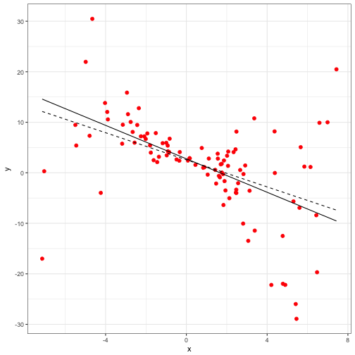
Random X (Model II Regression)
- Both \(X \) and \(Y \) chosen haphazardly or at random
- Model II Regression and the approach is controversial
- If the purpose of regression is prediction, then OLS
- If the purpose of regression is mechanisms, then not OLS (?)
- error variability associated with both Y \( \sigma_{\epsilon}^2 \) and X \( \sigma_{\gamma}^2 \) and the OLS estimate of \( \beta_1 \) is biased towards zero
- Major axis (MA) regression fits line minimizing the sum of squared perpendicular distances from each observation to the fitted line
- \( \sigma_{\epsilon}^2 \) = \( \sigma_{\gamma}^2 \)
- Reduced major axis (RMA) regression or standard major axis (SMA) regression is fitted by minimizing the sum of areas of the triangles formed by vertical and horizontal lines from each observation to the fitted line
- \( \sigma_{\epsilon}^2 \propto \sigma_x^2 \) and \( \sigma_{\gamma}^2 \propto \sigma_y^2\)
 # install.packages('lmodel2')

 data(mod2ex2)

Ex2.res <- lmodel2(Prey ~ Predators, data=mod2ex2, "relative", "relative", 99)
Ex2.res
##
## Model II regression
##
## Call: lmodel2(formula = Prey ~ Predators, data = mod2ex2, range.y
## = "relative", range.x = "relative", nperm = 99)
##
## n = 20 r = 0.8600787 r-square = 0.7397354
## Parametric P-values: 2-tailed = 0.000001161748 1-tailed = 0.0000005808741
## Angle between the two OLS regression lines = 5.106227 degrees
##
## Permutation tests of OLS, MA, RMA slopes: 1-tailed, tail corresponding to sign
## A permutation test of r is equivalent to a permutation test of the OLS slope
## P-perm for SMA = NA because the SMA slope cannot be tested
##
## Regression results
## Method Intercept Slope Angle (degrees) P-perm (1-tailed)
## 1 OLS 20.02675 2.631527 69.19283 0.01
## 2 MA 13.05968 3.465907 73.90584 0.01
## 3 SMA 16.45205 3.059635 71.90073 NA
## 4 RMA 17.25651 2.963292 71.35239 0.01
##
## Confidence intervals
## Method 2.5%-Intercept 97.5%-Intercept 2.5%-Slope 97.5%-Slope
## 1 OLS 12.490993 27.56251 1.858578 3.404476
## 2 MA 1.347422 19.76310 2.663101 4.868572
## 3 SMA 9.195287 22.10353 2.382810 3.928708
## 4 RMA 8.962997 23.84493 2.174260 3.956527
##
## Eigenvalues: 269.8212 6.418234
##
## H statistic used for computing C.I. of MA: 0.006120651- Simulated comparisons of OLS, MA and RMA regression analyses when X is random indicated:
- RMA estimate of \( /beta_1 )\ is less biased than the MA estimate
- If the error variability in X is more than ~ a third of the error variability in Y, then RMA is the preferred method; otherwise OLS is acceptable
Robust regression
- Limitation of OLS is that the estimates of model parameters, and therefore subsequent hypothesis tests, can be sensitive to distributional assumptions and affected by outlying observations
Least absolute deviance (LAD)
- Minimize the sum of absolute values of the residuals rather than the sum of squared residuals
- not squaring the residuals, extreme observations have less influence on the fitted model
M-estimator
- M-estimators involve minimizing the sum of some function of \( e_i \)
- Huber M-estimators, described earlier, weight the observations differently depending how far they are from the central tendency
crime_data <- read_csv(getURL("https://raw.githubusercontent.com/chrischizinski/SNR_R_Group/master/data/crime_data.csv"))
head(crime_data)
## # A tibble: 6 × 9
## sid state crime murder pctmetro pctwhite pcths poverty single
## <dbl> <chr> <int> <dbl> <dbl> <dbl> <dbl> <dbl> <dbl>
## 1 1 ak 761 9.0 41.8 75.2 86.6 9.1 14.3
## 2 2 al 780 11.6 67.4 73.5 66.9 17.4 11.5
## 3 3 ar 593 10.2 44.7 82.9 66.3 20.0 10.7
## 4 4 az 715 8.6 84.7 88.6 78.7 15.4 12.1
## 5 5 ca 1078 13.1 96.7 79.3 76.2 18.2 12.5
## 6 6 co 567 5.8 81.8 92.5 84.4 9.9 12.1crime_mod <- lm(crime ~ single, data = crime_data)
summary(crime_mod)##
## Call:
## lm(formula = crime ~ single, data = crime_data)
##
## Residuals:
## Min 1Q Median 3Q Max
## -767.42 -116.82 -20.58 125.28 719.70
##
## Coefficients:
## Estimate Std. Error t value Pr(>|t|)
## (Intercept) -1362.53 186.23 -7.316 2.15e-09 ***
## single 174.42 16.17 10.788 1.53e-14 ***
## ---
## Signif. codes: 0 '***' 0.001 '**' 0.01 '*' 0.05 '.' 0.1 ' ' 1
##
## Residual standard error: 242.5 on 49 degrees of freedom
## Multiple R-squared: 0.7037, Adjusted R-squared: 0.6977
## F-statistic: 116.4 on 1 and 49 DF, p-value: 1.529e-14crime_fit <- data.frame(state = crime_data$state, augment(crime_mod))ggplot(data = crime_fit) +
geom_line(aes(x = single, y = .fitted), color = "red") +
geom_point(aes(x = single, y = crime, colour = .std.resid ), size = 2) +
geom_text(aes(x = single, y = crime, label = state ), hjust = 0, vjust = 1) +
scale_colour_continuous(low = "red", high = "blue") +
theme_bw()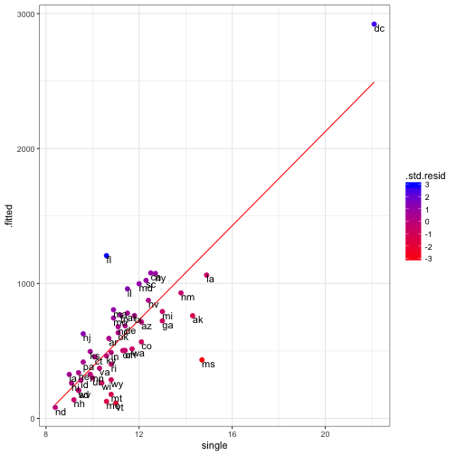
mod_huber <- rlm(crime ~ single, data = crime_data)
summary(mod_huber)
##
## Call: rlm(formula = crime ~ single, data = crime_data)
## Residuals:
## Min 1Q Median 3Q Max
## -797.489 -130.956 -9.108 127.019 716.664
##
## Coefficients:
## Value Std. Error t value
## (Intercept) -1429.3999 164.1623 -8.7072
## single 181.0128 14.2519 12.7010
##
## Residual standard error: 192.9 on 49 degrees of freedomhuber_dat<-data.frame(state = crime_data$state, augment(mod_huber), weight = mod_huber$w)ggplot(data = huber_dat) +
geom_line(aes(x = single, y = .fitted), color = "red") +
geom_point(aes(x = single, y = crime, colour = weight ), size = 2) +
geom_text(aes(x = single, y = crime, label = state ), hjust = 0, vjust = 1) +
scale_colour_continuous(low = "red", high = "blue") +
theme_bw()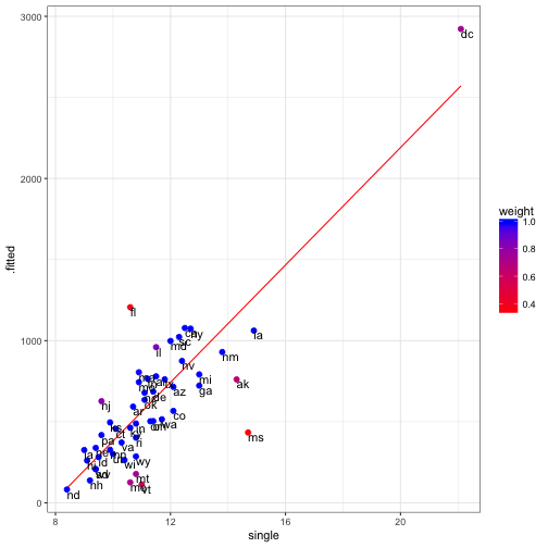
Rank-based regression
- Does not assume any specific distribution of the error terms but still fits the usual linear regression model
- Transformations are either ineffective or misrepresent the underlying biological process
# install.packages("Rfit")

mod_rank <- rfit(crime ~ single, data = crime_data)
summary(mod_rank)
## Call:
## rfit.default(formula = crime ~ single, data = crime_data)
##
## Coefficients:
## Estimate Std. Error t.value p.value
## (Intercept) -1400.923 182.905 -7.6593 6.362e-10 ***
## single 176.538 15.861 11.1305 5.109e-15 ***
## ---
## Signif. codes: 0 '***' 0.001 '**' 0.01 '*' 0.05 '.' 0.1 ' ' 1
## Overall Wald Test: 123.8871 p-value: 0Relationship between regression and correlation
- Simple correlation analysis is used when we seek to measure the strength of the linear relationship (the correlation coefficient) between the two variables
- Regression analysis is used when we can biologically distinguish a response \(( Y \) to a predictor variable \( X \)
- We can construct a model relating \(( Y \) to \( X \) and this to predict \(( Y \) from \( X \)