Estimation of parameters

Like determining population parameters , we often want to calculate the parameters in our regression models. There are two basic procedures that are often used to determine those. These sections are only meant to be illustrative and not comprehensive into the topic.

I based these illustrations heavily on the material from the Ecological Detective: Confronting Models with Data. I highly encourage you to read this book and follow along with the psuedo code in the book.

Sum of squares (Ordinary Least Squares [OLS])

Simplest method of estimating parameters.

Several selling points:

Simple, no assumptions about the uncertainty
Long history of use in science
Computational methods allow us to do remarkable calculations

library(ggplot2)
set.seed(456789)

fake_data<-data.frame(x = rpois(30, 5))
fake_data$y = fake_data$x *2 + rnorm(30, sd = 2)

ggplot(data = fake_data) + 
  geom_point(aes(x = x, y = y), size = 2) +
  theme_bw()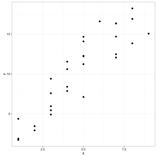

plot of chunk unnamed-chunk-1

start.val <- -2
max.val <- 6

poss.vals <- seq(start.val,max.val, by= 0.01)

length(poss.vals)

## [1] 801

SS_stor<-data.frame(poss.val = poss.vals, SS = NA)

for( i in 1:length(poss.vals)){
  pred.vals<- fake_data$x * poss.vals[i]
  
  SS_stor$SS[i] <- sum((pred.vals - fake_data$y)^2)
}

beta_val<-SS_stor$poss.val[which(SS_stor$SS == min(SS_stor$SS))]

ggplot(data=SS_stor) +
  geom_line(aes(x = poss.vals, y = SS), size = 1) +
  geom_vline(aes(xintercept = beta_val), colour = "red", linetype = "dashed") +
  labs(x = "Possible values", y = "Sum of squares") +
  scale_x_continuous(breaks = seq(start.val,max.val, by = 0.5)) +
  theme_bw()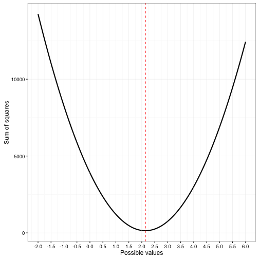

plot of chunk unnamed-chunk-2

beta_pred <- data.frame(x = min(fake_data$x):max(fake_data$x))
beta_pred$fit.y <- beta_pred$x * beta_val

ggplot() + 
  geom_point(data = fake_data, aes(x = x, y = y), size = 2) +
  geom_line(data = beta_pred, aes(x = x, y = fit.y), colour="red") +
  theme_bw()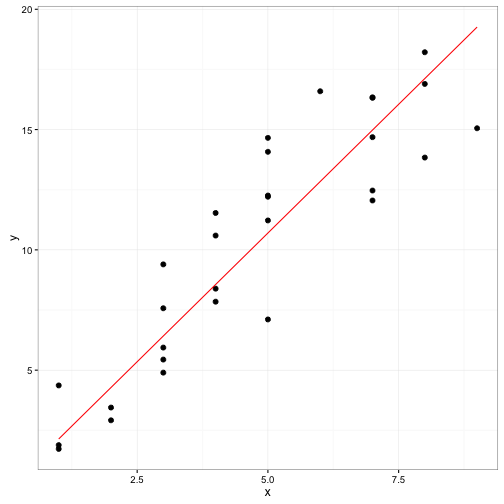

plot of chunk unnamed-chunk-3

What if we have two parameters?

set.seed(345678)

fake_data2<-data.frame(x1 = rpois(30, 5), x2 = rpois(30, 2))
fake_data2$y = fake_data2$x1 *2 + rnorm(30, sd = 2) + fake_data2$x2 *-4 + rnorm(30, sd = 2)

Use the above approach to estimate the values for the two parameters.

Click here for answer

Maximum likelihood

Given a set of observations from the population, we can find estimates of one (or many) parameters that maximize the liklihood of observing those data. The likelihood function provides the likelihood of the observed data for all possible values of the parameter we are trying to estimate.

This approach allows us to incorporate some of the uncertainty based on probability distributions. For example, if the deviations of the data from the average follow a normal distribution, then it can be assumed that the uncertainty is normally distributed.

This approach allows us to develop confidence bounds around our parameters that we could not do in the sum of squares approach.

Likelihood and Maximum Likelihood

The probability of observing the data $ Y_i $ given a particular parameter value $ p $ is:

$Pr(Y_i | p)$

The subscript on Y, indicates that there are many possible outcomes but only one parameter $ p $. Thus we can ask, “Given these data, how likely are the possible hypothesis?”

$L \{ data | hypothesis \}$

$L \{ Y | p_m \}$

Notice the difference from the previous equation. In the likelihood function we have one observation but numerous potential hypotheses or parameter values. The key difference between likelihood and probability is that with the probability the hypothesis is known and data are unknown, whereas the likelihood the data are known and the hypotheses are unknown.

Thus there are parameter values that are more likely than others.

The parameter that makes the likelihood as large as possible is the maximum likelihood estimate (MLE). Generally likelihoods are very small values and thus the log likelihood is used and to make it analogous to sum of squares we use the negative value of that. So the best fit parameter value will be the negative, log likelihood.

As an example, consider the heights of ten people in cm. We can assume that height is normally distributed with a standard deviation of 10 cm.

height_data <- data.frame(ind = 1:10, height = c(171, 168, 180, 190, 169, 172, 162, 181, 181, 177) )

height_data

##    ind height
## 1    1    171
## 2    2    168
## 3    3    180
## 4    4    190
## 5    5    169
## 6    6    172
## 7    7    162
## 8    8    181
## 9    9    181
## 10  10    177

The likelihood for the true mean of the population can be given as:

$L\{Y | p_m \} = \frac{1}{10 \sqrt{2 \pi}} exp \left( - \frac{(Y - m)^2}{200} \right)$

and the negative log-likelihood for 10 of the ten heights is:

$L\{Y | p_m \} = n[\log(10) + \frac{1}{2}\log(2 \pi) ] + \sum_{i=1}^n \frac{(Y_i - m)^2}{200}$

m<- seq(160, 200, by= 0.25) # mean height

data_stor<-data.frame(m = m, ll = NA)

for(i in 1:length(m)){
  
  ll <- 10*(log(10) + 1/2*log(2*pi)) + sum((height_data$height - m[i])^2)/200
  
  data_stor$ll[i] <- ll
  }

ggplot() +
  geom_line(data =data_stor, aes(x = m, y = ll), size = 1, colour = "blue" ) +
  scale_x_continuous(breaks = seq(160, 200, by = 5)) +
  theme_bw()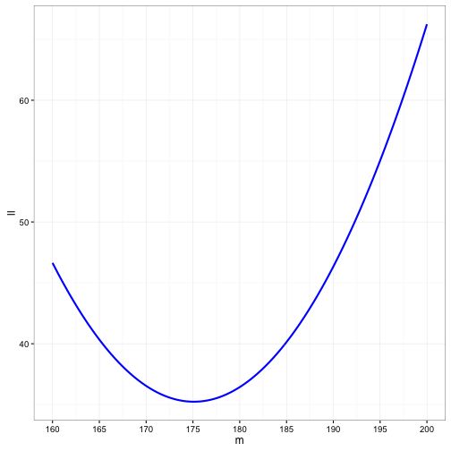

plot of chunk unnamed-chunk-7

And to find that value:

data_stor[which(data_stor$ll == min(data_stor$ll)),]

##      m       ll
## 61 175 35.24024

This is an overly simplified description of using likelihood to estimate parameters. In all reality, it often requires calculus or complex iterative algorithms to determine the value that maximizes the likelihood function.