The RMarkdown file for this lesson can be found here
This lesson will follow Chapter 3 in Quinn and Keough (2002).
Statistical hypothesis testing
In the biological sciences, among other sciences, it is not often enough to just collect information on the central tendency of a population or parameter. We often want to compare estimates among populations or against environmental variables. Perhaps not surprisingly, there is still controversy on how this should be approached and the philosophies behind the approach. Chapter two in the the Ecological Detective: Confronting Models with Data has a great synopsis of these.
Classical hypothesis testing
There are two basic concepts:
- State a statistical null hypothesis $H_0$
- generally a statement of no difference or no relationship
- Popperian falsification: science progresses by testing and falsifying hypothesis. Rejection of $H_0$ is equivalent to falsifying
- We must choose a test statistic to test the $H_0$
- a test statistic is a random variable and can be described from a probability distribution
Fisher’s approach to hypothesis testing
- Construct a $H_0$
- Choose a test statistic that measures deviation from $H_0$ and has a known sampling distribution
- Collect the data by one or more random samples from the population and compare the test statistic to its sampling distribution
- Determine the P-value
- the associated of obtaining our sample value of the statistic, or one more extreme, if $H_0$ is true
- Reject $H_0$ if P is small; retain $H_0$ otherwise
- P value can be viewed as the “strength of evidence” against $H_0$
- Fixed significance levels (i.e., 0.05) are too restrictive
Neyman and Pearson approach to hypothesis testing
- Level of signficance set prior to data collection (fixed level testing)
- Significance level is interpretted as the proportion of times the $H_0$ would be wrongly rejected using this decision rule if the experiment were repeated many times and $H_0$ were actually true
- Emphasized making decision about $H_0$ and the errors associated with it, whereas Fisher emphasized measuring the evidence against $H_0$
- Alternative hypothesis $H_A$, which is the alternate if $H_0$ is false (Fisher opposed this idea)
- Type I error (long-run probability of falsely rejecting $H_0$), Type II error (long-run probability of falsely not rejecting $H_0$)
The Hybrid approach
- Specify $H_0$, $H_A$, and test statistic
- Specify a priori significance level that is the long-run frequency of Type I errors ($\alpha$) that you are willing to accept
- Collect the data via random sampling and calculate test statistic
- Compare test statistic to its sampling distribution, assuming $H_0$ is true
- If the probability is less than specified significance level, then conclude that $H_0$ is false and reject
- If the probability is greater than the specified significance level, then conclude there is no evidence that $H_0$ is false and retain
Hypothesis tests for a single population
We will illustrate this with a simple, single-parametr t test. t tests can be used to single population parameters or between two population parameters.
The general form of the t statistic is:
where St is the value from our sample, $\Theta$ is the population value against which the sample statistic is to be tested and $S_St$ is the estimated standard error of the sample statistic.
set.seed(12345)

data_of_pop <- data.frame(ind = 1:100, height = rnorm(1000, mean = 65, sd = 3.5))
If you are using a $H_0$ of $\mu = 0$ and $H_A$ of $\mu \neq 0$
- Take a random sample from
data_of_popof 100 individuals. - Calculate your t statistic
- Compare your t statistic with the sampling distribution of t at $\alpha = 0.05$
sub_sample <- data_of_pop[sample(1:nrow(data_of_pop), 100, replace=FALSE),]

mean_height <- mean(sub_sample$height)
sd_height <- sd(sub_sample$height)
se_height <- sd_height/sqrt(100)

t = (mean_height - 0)/se_height

qt(0.975, df = 100-1)
## [1] 1.984217#Reject H0 if t is > tcrit
t.test(sub_sample$height)##
## One Sample t-test
##
## data: sub_sample$height
## t = 183.39, df = 99, p-value < 2.2e-16
## alternative hypothesis: true mean is not equal to 0
## 95 percent confidence interval:
## 64.74261 66.15894
## sample estimates:
## mean of x
## 65.45077One or two-tailed tests
Most cases in biology, $H_0$ is that there is no difference in means) and the $H_A$ can be in either direction. This is two-tailed because arge values of the test statistic at either end of the sampling distribution will result in rejection of $H_0$. We can specify a test though that $H_A$ can be that the mean is lower or greater. This is a one-tailed test.
##
## Attaching package: 'gridExtra'
## The following object is masked from 'package:dplyr':
##
## combinegrid.arrange(plota, plotb, ncol=1, left = textGrob("Density", gp = gpar(fontsize = 18), rot = 90),
bottom =textGrob("t value", gp = gpar(fontsize = 18)) )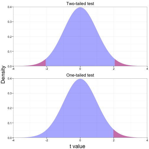
Hypothesis tests of two populations
Differences between two populations
If we have random samples from two populations then we can compare the means of the populations. The $H_0$ becomes $\mu_1 = \mu_2$
The calculation of the t statistic is similar to how we calculated it from the single population, except the standard error is the standard error of the differences between the populations
This is similar to the t test from the single population.
Our $H_0$ is that there is no difference between the population means so $\mu_1 - \mu_2 = 0$.
To calculate the standard error of the differences we use:
And in this case our $df = n_1 +n_2 -2$.
set.seed(4321)

test.group<-rbind(data.frame(grp = "A",value = rnorm(15, mean = 22, sd = 3)),
                  data.frame(grp = "B",value = rnorm(20, mean = 30, sd = 3)))

# independent 2-group t-test
t.test(test.group$value~test.group$grp, var.equal = TRUE) # where y is numeric and x is a binary factor, var.equal = FALSE is the default
##
## Two Sample t-test
##
## data: test.group$value by test.group$grp
## t = -8.7323, df = 33, p-value = 4.301e-10
## alternative hypothesis: true difference in means is not equal to 0
## 95 percent confidence interval:
## -9.306298 -5.789243
## sample estimates:
## mean in group A mean in group B
## 22.34888 29.89665t.test(test.group$value~test.group$grp, var.equal = FALSE) # where y is numeric and x is a binary factor##
## Welch Two Sample t-test
##
## data: test.group$value by test.group$grp
## t = -8.6676, df = 29.443, p-value = 1.34e-09
## alternative hypothesis: true difference in means is not equal to 0
## 95 percent confidence interval:
## -9.327604 -5.767937
## sample estimates:
## mean in group A mean in group B
## 22.34888 29.89665 # Note the difference in the df
# independent 2-group t-test
t.test(test.group$value[test.group$grp =="A"],test.group$value[test.group$grp =="B"]) # where y1 and y2 are numeric##
## Welch Two Sample t-test
##
## data: test.group$value[test.group$grp == "A"] and test.group$value[test.group$grp == "B"]
## t = -8.6676, df = 29.443, p-value = 1.34e-09
## alternative hypothesis: true difference in means is not equal to 0
## 95 percent confidence interval:
## -9.327604 -5.767937
## sample estimates:
## mean of x mean of y
## 22.34888 29.89665Paired T-tests
Two data samples are matched if they come from repeated observations of the same subject. Using the paired t-test, we can obtain an interval estimate of the difference of the population means.
library(MASS)

head(immer)
## Loc Var Y1 Y2
## 1 UF M 81.0 80.7
## 2 UF S 105.4 82.3
## 3 UF V 119.7 80.4
## 4 UF T 109.7 87.2
## 5 UF P 98.3 84.2
## 6 W M 146.6 100.4t.test(immer$Y1, immer$Y2, paired=TRUE) ##
## Paired t-test
##
## data: immer$Y1 and immer$Y2
## t = 3.324, df = 29, p-value = 0.002413
## alternative hypothesis: true difference in means is not equal to 0
## 95 percent confidence interval:
## 6.121954 25.704713
## sample estimates:
## mean of the differences
## 15.91333Resampling
# install.packages("boot")
library(boot)
##
## Attaching package: 'boot'## The following object is masked from 'package:psych':
##
## logitorg_counts = data.frame(grp1=rpois(30, lambda = 15),
grp2=rpois(30, lambda = 20))
head(org_counts)## grp1 grp2
## 1 12 19
## 2 15 21
## 3 13 19
## 4 18 19
## 5 22 12
## 6 13 20diff.means <- function(x, w){
m1 = mean(x$grp1[w])
m2 = mean(x$grp2[w])
c(m1 - m2)
}
boot_result<-boot(org_counts, diff.means, R = 5000)
boot_result##
## ORDINARY NONPARAMETRIC BOOTSTRAP
##
##
## Call:
## boot(data = org_counts, statistic = diff.means, R = 5000)
##
##
## Bootstrap Statistics :
## original bias std. error
## t1* -3.766667 0.01816 1.365001names(boot_result)## [1] "t0" "t" "R" "data" "seed"
## [6] "statistic" "sim" "call" "stype" "strata"
## [11] "weights"sum(abs(boot_result$t) >= abs(boot_result$t0))/length(boot_result$t)## [1] 0.4966data2= data.frame(values=boot_result$t )
ggplot(data = data2) +
geom_histogram(aes(x = abs(values)), bins =50) +
geom_vline(aes(xintercept = abs(boot_result$t0)), colour = "red") +
theme_bw()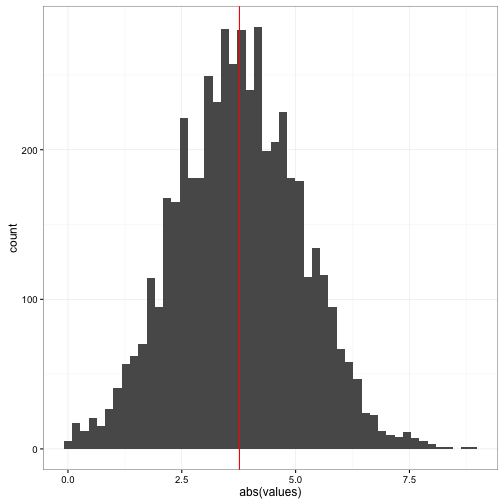
t.test(org_counts$grp1,org_counts$grp2)##
## Welch Two Sample t-test
##
## data: org_counts$grp1 and org_counts$grp2
## t = -3.0793, df = 55.706, p-value = 0.003219
## alternative hypothesis: true difference in means is not equal to 0
## 95 percent confidence interval:
## -6.217370 -1.315964
## sample estimates:
## mean of x mean of y
## 16.20000 19.96667Rank-based non-parametric tests
Mann– Whitney–Wilcoxon test
- Rank all the observations, ignoring the groups. Tied observations get the average of their ranks.
- Calculate the sum of the ranks for both samples. If the H0 is true, we would expect a similar mixture of ranks in both samples (Sprent 1993).
- Compare the smaller rank sum to the probability distribution of rank sums, based on repeated randomization of observations to groups, and test in the usual manner.
- For larger sample sizes, the probability distribution of rank sums approximates a normal distribution and the z statistic can be used.
The H0 being tested is that the two samples come from populations with identical distributions against the HA that the samples come from populations which differ only in location (mean or median)
wilcox.test(mpg ~ am, data=mtcars) ## Warning in wilcox.test.default(x = c(21.4, 18.7, 18.1, 14.3, 24.4, 22.8, :
## cannot compute exact p-value with ties##
## Wilcoxon rank sum test with continuity correction
##
## data: mpg by am
## W = 42, p-value = 0.001871
## alternative hypothesis: true location shift is not equal to 0Wilcoxon signed-rank test to test the H0 that the two sets of observations come from the same population against the HA that the pop- ulations differ in location (mean or median).
- Calculate the difference between the observations for each pair, noting the sign of each difference. If H0 is true, we would expect roughly equal numbers of and signs.
- Calculate the sum of the positive ranks and the sum of the negative ranks.
- Compare the smaller of these rank sums to the probability distribution of rank sums, based on randomization, and test in the usual manner.
- For larger sample sizes, the probability distribution of rank sums follows a normal distribution and the z statistic can be used
head(immer) ## Loc Var Y1 Y2
## 1 UF M 81.0 80.7
## 2 UF S 105.4 82.3
## 3 UF V 119.7 80.4
## 4 UF T 109.7 87.2
## 5 UF P 98.3 84.2
## 6 W M 146.6 100.4wilcox.test(immer$Y1, immer$Y2, paired=TRUE) ## Warning in wilcox.test.default(immer$Y1, immer$Y2, paired = TRUE): cannot
## compute exact p-value with ties##
## Wilcoxon signed rank test with continuity correction
##
## data: immer$Y1 and immer$Y2
## V = 368.5, p-value = 0.005318
## alternative hypothesis: true location shift is not equal to 0Lets put this into practice:
- Load the
warddataset from theChap3folder on the github repository.
Ward & Quinn (1988) studied aspects of the ecology of the intertidal predatory gastropod Lepsiella vinosa on a rocky shore in southeastern Australia. L. vinosa occurred in two distinct zones on this shore: a high-shore zone dominated by small grazing gastropods Littorina spp. and a mid-shore zone dominated by beds of the mussels Xenostrobus pulex and Brachidontes rostratus. Both gastropods and mussels are eaten by L. vinosa. Other data indicated that rates of energy consumption by L. vinosa were much greater in the mussel zone. Ward & Quinn (1988) were interested in whether there were any differences in fecundity of L. vinosa, especially the number of eggs per capsule, between the zones.
- Load the
furnessdataset from theChap3folder on the github repository.
Furness & Bryant (1996) studied energy budgets of breeding northern fulmars (Fulmarus glacialis) in Shetland. As part of their study, they recorded various characteristics of individually labeled male and female fulmars. We will focus on differences between sexes in metabolic rate.
- Load the
elgardataset from theChap3folder on the github repository.
Elgar et al. (1996) studied the effect of lighting on the web structure of an orb- spinning spider. They set up wooden frames with two different light regimes (controlled by black or white mosquito netting), light and dim. A total of 17 orb spiders were allowed to spin their webs in both a light frame and a dim frame, with six days’ “rest” between trials for each spider, and the vertical and horizontal diameter of each web was measured. Whether each spider was allocated to a light or dim frame first was randomized. The null hypotheses were that the two variables (vertical diameter and horizontal diameter of the orb web) were the same in dim and light conditions.
- Calculate n, Mean, Median, Standard deviation, SE of the mean, 95% CI of mean for each group
- Graphically evaluate the variance among the groups
- Choose the correct type of test to test differences between each group.
Click here for answers