Recreating Figure 2.1 in Ecological Detective
There are many different hypotheses that can explain the basic relationship between two variables. Figure 2.1 in the Ecologial Detective suggest 4 possible models. The models have no parameter values. Try to iteratively find the parameter values to get your figure to look like the one in Figure 2.1.
S <- seq(1,15, by = 1)  # 1:15
Null_hypothesis<- 2.5

our_data <- data.frame(S = S, Null = Null_hypothesis)
our_data$Model_A <- 0.5 *S
our_data$Model_B <- (0.9 *S)/(1 + 0.1*S)
our_data$Model_C <- 1.8 *S * exp(-0.18*S)

plot_labels = data.frame(x = c(14,14,8, 4), y = c(7.5,5.5,2.75,3.5), labels = c("Model A", "Model B", "NULL", "Model C"))


ggplot() +
  geom_line(data = our_data,aes(x = S, y = Null), colour="black") +
  geom_line(data = our_data,aes(x = S, y = Model_A), colour="blue") +
  geom_line(data = our_data,aes(x = S, y = Model_B), colour="green") +
  geom_line(data = our_data,aes(x = S, y = Model_C), colour="red") +
  geom_text(data = plot_labels, aes(x=x, y= y, label = labels)) +
  coord_cartesian(ylim = c(0,9), xlim = c(0, 16), expand = FALSE) +
  scale_x_continuous(breaks = seq(0,16,by=2)) +
  scale_y_continuous(breaks = seq(1,8,by=1)) +
  labs(x = "Flock size", y = "Consumption rate") +
  theme_bw()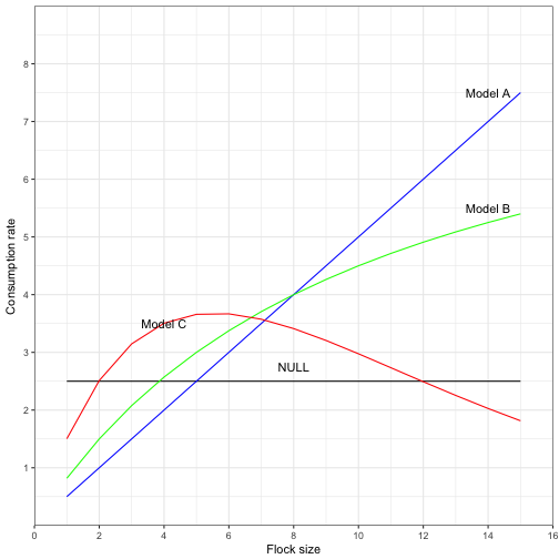
Probability and probability models
- Ecological data (and most other kinds of data) involve different levels of randomness
- Most models represent the mean of the population
-
Comparing models requires understanding the probability of individual observations (based on the distribution)
- Most people understand the normal or Gaussian distribution, but htere are many, many different types of distributions
WORD OF ADVICE: Always plot your data
fish_data <- read_csv("https://raw.githubusercontent.com/chrischizinski/MWFWC_FishR/master/CourseMaterial/data/wrkshp_data.csv")## Parsed with column specification:
## cols(
## .default = col_character(),
## WaterbodyCode = col_integer(),
## Area = col_integer(),
## MethodCode = col_integer(),
## surveydate = col_datetime(format = ""),
## Station = col_integer(),
## Effort = col_integer(),
## SpeciesCode = col_integer(),
## LengthGroup = col_integer(),
## FishCount = col_integer(),
## FishLength = col_integer(),
## FishWeight = col_integer(),
## Age = col_integer(),
## Edge = col_integer(),
## Annulus1 = col_integer(),
## Annulus2 = col_integer(),
## Annulus3 = col_integer(),
## Annulus4 = col_integer(),
## Annulus5 = col_integer(),
## Annulus6 = col_integer(),
## Annulus7 = col_integer()
## # ... with 2 more columns
## )## See spec(...) for full column specifications.glimpse(fish_data)## Observations: 16,527
## Variables: 43
## $ WaterbodyCode <int> 4113, 4113, 4113, 4113, 4113, 4113, 4113, 4113, ...
## $ Area <int> 0, 0, 0, 0, 0, 0, 0, 0, 0, 0, 0, 0, 0, 0, 0, 0, ...
## $ MethodCode <int> 21, 21, 21, 21, 21, 21, 21, 21, 21, 21, 21, 21, ...
## $ surveydate <dttm> 2014-10-29 05:00:00, 2014-10-29 05:00:00, 2014-...
## $ Station <int> 1, 1, 1, 1, 1, 1, 1, 1, 1, 1, 2, 2, 2, 2, 2, 2, ...
## $ Effort <int> 1, 1, 1, 1, 1, 1, 1, 1, 1, 1, 1, 1, 1, 1, 1, 1, ...
## $ SpeciesCode <int> 730, 730, 730, 730, 730, 730, 730, 730, 730, 730...
## $ LengthGroup <int> 100, 120, 140, 150, 160, 170, 180, 190, 200, 210...
## $ FishCount <int> 1, 1, 1, 2, 2, 3, 6, 6, 3, 3, 2, 3, 2, 1, 2, 1, ...
## $ FishLength <int> NA, NA, NA, NA, NA, NA, NA, NA, NA, NA, NA, NA, ...
## $ FishWeight <int> NA, NA, NA, NA, NA, NA, NA, NA, NA, NA, NA, NA, ...
## $ Age <int> NA, NA, NA, NA, NA, NA, NA, NA, NA, NA, NA, NA, ...
## $ Edge <int> NA, NA, NA, NA, NA, NA, NA, NA, NA, NA, NA, NA, ...
## $ Annulus1 <int> NA, NA, NA, NA, NA, NA, NA, NA, NA, NA, NA, NA, ...
## $ Annulus2 <int> NA, NA, NA, NA, NA, NA, NA, NA, NA, NA, NA, NA, ...
## $ Annulus3 <int> NA, NA, NA, NA, NA, NA, NA, NA, NA, NA, NA, NA, ...
## $ Annulus4 <int> NA, NA, NA, NA, NA, NA, NA, NA, NA, NA, NA, NA, ...
## $ Annulus5 <int> NA, NA, NA, NA, NA, NA, NA, NA, NA, NA, NA, NA, ...
## $ Annulus6 <int> NA, NA, NA, NA, NA, NA, NA, NA, NA, NA, NA, NA, ...
## $ Annulus7 <int> NA, NA, NA, NA, NA, NA, NA, NA, NA, NA, NA, NA, ...
## $ Annulus8 <int> NA, NA, NA, NA, NA, NA, NA, NA, NA, NA, NA, NA, ...
## $ Annulus9 <int> NA, NA, NA, NA, NA, NA, NA, NA, NA, NA, NA, NA, ...
## $ Annulus10 <chr> NA, NA, NA, NA, NA, NA, NA, NA, NA, NA, NA, NA, ...
## $ Annulus11 <chr> NA, NA, NA, NA, NA, NA, NA, NA, NA, NA, NA, NA, ...
## $ Annulus12 <chr> NA, NA, NA, NA, NA, NA, NA, NA, NA, NA, NA, NA, ...
## $ Annulus13 <chr> NA, NA, NA, NA, NA, NA, NA, NA, NA, NA, NA, NA, ...
## $ Annulus14 <chr> NA, NA, NA, NA, NA, NA, NA, NA, NA, NA, NA, NA, ...
## $ Annulus15 <chr> NA, NA, NA, NA, NA, NA, NA, NA, NA, NA, NA, NA, ...
## $ Annulus16 <chr> NA, NA, NA, NA, NA, NA, NA, NA, NA, NA, NA, NA, ...
## $ Annulus17 <chr> NA, NA, NA, NA, NA, NA, NA, NA, NA, NA, NA, NA, ...
## $ Annulus18 <chr> NA, NA, NA, NA, NA, NA, NA, NA, NA, NA, NA, NA, ...
## $ Annulus19 <chr> NA, NA, NA, NA, NA, NA, NA, NA, NA, NA, NA, NA, ...
## $ Annulus20 <chr> NA, NA, NA, NA, NA, NA, NA, NA, NA, NA, NA, NA, ...
## $ Annulus21 <chr> NA, NA, NA, NA, NA, NA, NA, NA, NA, NA, NA, NA, ...
## $ Annulus22 <chr> NA, NA, NA, NA, NA, NA, NA, NA, NA, NA, NA, NA, ...
## $ Annulus23 <chr> NA, NA, NA, NA, NA, NA, NA, NA, NA, NA, NA, NA, ...
## $ Annulus24 <chr> NA, NA, NA, NA, NA, NA, NA, NA, NA, NA, NA, NA, ...
## $ Annulus25 <chr> NA, NA, NA, NA, NA, NA, NA, NA, NA, NA, NA, NA, ...
## $ Annulus26 <chr> NA, NA, NA, NA, NA, NA, NA, NA, NA, NA, NA, NA, ...
## $ Annulus27 <chr> NA, NA, NA, NA, NA, NA, NA, NA, NA, NA, NA, NA, ...
## $ Annulus28 <chr> NA, NA, NA, NA, NA, NA, NA, NA, NA, NA, NA, NA, ...
## $ Annulus29 <chr> NA, NA, NA, NA, NA, NA, NA, NA, NA, NA, NA, NA, ...
## $ Annulus30 <chr> NA, NA, NA, NA, NA, NA, NA, NA, NA, NA, NA, NA, ...fish_data %>%
select(WaterbodyCode:Age) %>%
mutate(Age = as.numeric(Age)) %>%
filter(!is.na(Age),
WaterbodyCode == 4999,
SpeciesCode %in% c(780)) -> FishAge
glimpse(FishAge)## Observations: 82
## Variables: 12
## $ WaterbodyCode <int> 4999, 4999, 4999, 4999, 4999, 4999, 4999, 4999, ...
## $ Area <int> 0, 0, 0, 0, 0, 0, 0, 0, 0, 0, 0, 0, 0, 0, 0, 0, ...
## $ MethodCode <int> 21, 21, 21, 21, 21, 21, 21, 21, 21, 21, 21, 21, ...
## $ surveydate <dttm> 2013-09-24 05:00:00, 2013-09-24 05:00:00, 2013-...
## $ Station <int> 2, 2, 2, 2, 4, 4, 1, 1, 2, 2, 2, 2, 2, 2, 2, 2, ...
## $ Effort <int> 1, 1, 1, 1, 1, 1, 1, 1, 1, 1, 1, 1, 1, 1, 1, 1, ...
## $ SpeciesCode <int> 780, 780, 780, 780, 780, 780, 780, 780, 780, 780...
## $ LengthGroup <int> NA, NA, NA, NA, NA, NA, NA, NA, NA, NA, NA, NA, ...
## $ FishCount <int> NA, NA, NA, NA, NA, NA, NA, NA, NA, NA, NA, NA, ...
## $ FishLength <int> 248, 232, 195, 264, 262, 258, 96, 256, 233, 243,...
## $ FishWeight <int> 198, 154, 104, 242, 230, 210, 8, 218, 172, 168, ...
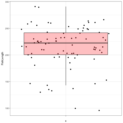
## $ Age <dbl> 7, 3, 2, 4, 6, 5, 1, 4, 5, 6, 5, 3, 3, 3, 3, 3, ...Let’s look at distribution plots of FishLength and Age
ggplot(data = FishAge) +
  geom_histogram(aes(x = Age), binwidth = 1, fill = "green", colour = "black") +
  theme_bw()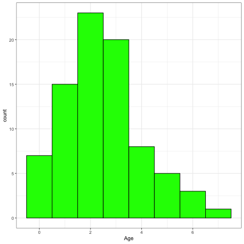
ggplot(data = FishAge,aes(x = Age)) +
  geom_histogram(aes(y = ..density..),binwidth = 1, fill = "green", colour = "black") +
  geom_density(colour = "red", fill = "red", alpha = 0.5) +
  theme_bw()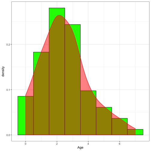
ggplot(data = FishAge) +
  geom_histogram(aes(x = FishLength), binwidth = 10, fill = "red", colour = "black" ) +
  theme_bw()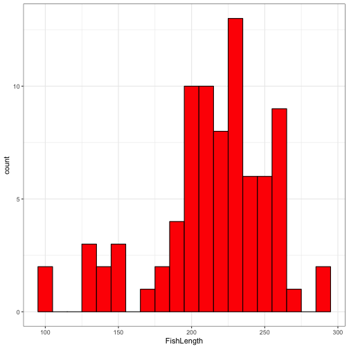
ggplot(data = FishAge) +
  geom_violin(aes(x = "", y = FishLength), fill = "red", colour = "black" ) +
  theme_bw()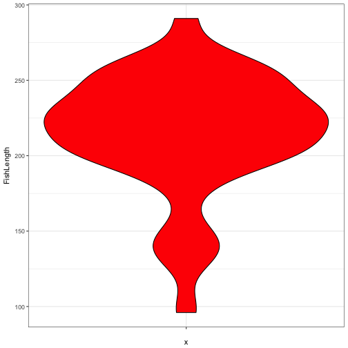
ggplot(data = FishAge) +
  geom_point(aes(x = "", y = FishLength), position = "jitter") +
  geom_boxplot(aes(x = "", y = FishLength), fill = "red", colour = "black", alpha = 0.25, outlier.colour = NA) +
  theme_bw()