Ecological Detective - Relationships and probability

Exploring the relationship between two variables

First lets bring in the data from the previous lesson

library(tidyverse)
library(broom)

fish_data <- read_csv("https://raw.githubusercontent.com/chrischizinski/MWFWC_FishR/master/CourseMaterial/data/wrkshp_data.csv")

## Parsed with column specification:
## cols(
##   .default = col_character(),
##   WaterbodyCode = col_integer(),
##   Area = col_integer(),
##   MethodCode = col_integer(),
##   surveydate = col_datetime(format = ""),
##   Station = col_integer(),
##   Effort = col_integer(),
##   SpeciesCode = col_integer(),
##   LengthGroup = col_integer(),
##   FishCount = col_integer(),
##   FishLength = col_integer(),
##   FishWeight = col_integer(),
##   Age = col_integer(),
##   Edge = col_integer(),
##   Annulus1 = col_integer(),
##   Annulus2 = col_integer(),
##   Annulus3 = col_integer(),
##   Annulus4 = col_integer(),
##   Annulus5 = col_integer(),
##   Annulus6 = col_integer(),
##   Annulus7 = col_integer()
##   # ... with 2 more columns
## )

## See spec(...) for full column specifications.

fish_data %>% 
  select(WaterbodyCode:Age) %>% 
  mutate(Age = as.numeric(Age)) %>% 
  filter(!is.na(Age),
         WaterbodyCode == 4999,
         SpeciesCode %in% c(780)) -> FishAge

Now lets plot the basic relationship between age and length of this species.

ggplot(data = FishAge) +
  geom_point(aes(x = Age, y = FishLength), size = 3, alpha = 0.35, colour = "red") +
  theme_bw()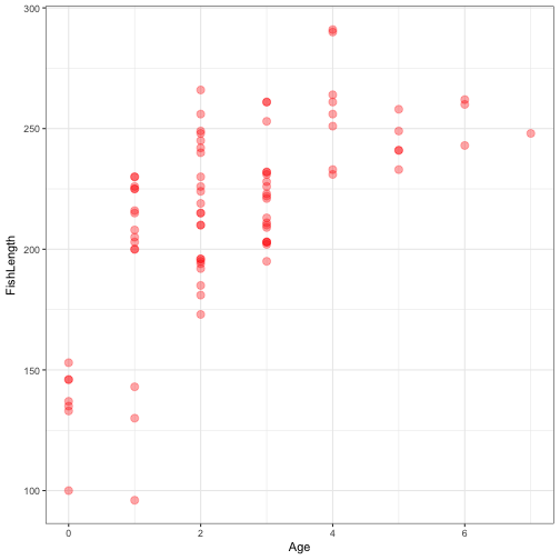

plot of chunk unnamed-chunk-3

How does fish age relate to fish length?

Linear
Polynomial
Logarithmic
Non-linear

# linear response
lm_mod <- lm(FishLength ~ Age, data = FishAge)
summary(lm_mod)

## 
## Call:
## lm(formula = FishLength ~ Age, data = FishAge)
## 
## Residuals:
##     Min      1Q  Median      3Q     Max 
## -94.265 -19.517   0.703  21.953  58.725 
## 
## Coefficients:
##             Estimate Std. Error t value Pr(>|t|)    
## (Intercept)  173.254      6.232  27.799  < 2e-16 ***
## Age           17.011      2.138   7.957  9.8e-12 ***
## ---
## Signif. codes:  0 '***' 0.001 '**' 0.01 '*' 0.05 '.' 0.1 ' ' 1
## 
## Residual standard error: 29.81 on 80 degrees of freedom
## Multiple R-squared:  0.4418,	Adjusted R-squared:  0.4348 
## F-statistic: 63.32 on 1 and 80 DF,  p-value: 9.797e-12

# polynomial response
poly_mod <- lm(FishLength ~ poly(Age,3), data = FishAge)
summary(poly_mod)

## 
## Call:
## lm(formula = FishLength ~ poly(Age, 3), data = FishAge)
## 
## Residuals:
##     Min      1Q  Median      3Q     Max 
## -92.393 -18.407  -1.423  19.566  49.441 
## 
## Coefficients:
##               Estimate Std. Error t value Pr(>|t|)    
## (Intercept)    215.366      3.011  71.527  < 2e-16 ***
## poly(Age, 3)1  237.206     27.266   8.700 4.13e-13 ***
## poly(Age, 3)2 -107.773     27.266  -3.953 0.000169 ***
## poly(Age, 3)3   38.539     27.266   1.413 0.161501    
## ---
## Signif. codes:  0 '***' 0.001 '**' 0.01 '*' 0.05 '.' 0.1 ' ' 1
## 
## Residual standard error: 27.27 on 78 degrees of freedom
## Multiple R-squared:  0.5447,	Adjusted R-squared:  0.5272 
## F-statistic:  31.1 on 3 and 78 DF,  p-value: 2.506e-13

# logarithmic

log_mod <- lm(FishLength ~ log(Age +1), data = FishAge)
summary(log_mod)

## 
## Call:
## lm(formula = FishLength ~ log(Age + 1), data = FishAge)
## 
## Residuals:
##     Min      1Q  Median      3Q     Max 
## -93.378 -17.928  -2.378  18.426  52.822 
## 
## Coefficients:
##              Estimate Std. Error t value Pr(>|t|)    
## (Intercept)   148.691      7.462  19.925  < 2e-16 ***
## log(Age + 1)   58.699      6.023   9.745 3.04e-15 ***
## ---
## Signif. codes:  0 '***' 0.001 '**' 0.01 '*' 0.05 '.' 0.1 ' ' 1
## 
## Residual standard error: 26.98 on 80 degrees of freedom
## Multiple R-squared:  0.5428,	Adjusted R-squared:  0.5371 
## F-statistic: 94.97 on 1 and 80 DF,  p-value: 3.039e-15

# non linear

nl_mod <- nls(FishLength ~ exp(a + Age*b), start = list(a = 0, b = 1), data = FishAge)
summary(nl_mod)

## 
## Formula: FishLength ~ exp(a + Age * b)
## 
## Parameters:
##   Estimate Std. Error t value Pr(>|t|)    
## a 5.191797   0.031178 166.522  < 2e-16 ***
## b 0.070687   0.009528   7.419  1.1e-10 ***
## ---
## Signif. codes:  0 '***' 0.001 '**' 0.01 '*' 0.05 '.' 0.1 ' ' 1
## 
## Residual standard error: 30.64 on 80 degrees of freedom
## 
## Number of iterations to convergence: 7 
## Achieved convergence tolerance: 0.00000223

Plot the curves to the data

newdata <- data.frame(Age = seq(0,8,by = 1))

lm_pred<- data.frame(model = "linear",augment(lm_mod, newdata = newdata))

poly_pred<- data.frame(model = "polynomial",augment(poly_mod, newdata = newdata))

log_pred<- data.frame(model = "log",augment(log_mod, newdata = newdata))
# log_pred$.fitted <- exp(log_pred$.fitted) 

nl_pred<- data.frame(model = "nonlinear",augment(nl_mod, newdata = newdata))
nl_pred$.se.fit<-NA

all.pred<- rbind(lm_pred,poly_pred,log_pred,nl_pred)

ggplot(data = FishAge) +
  geom_point(aes(x = Age, y = FishLength), size = 1, alpha = 0.35, colour = "red") +
  geom_line(data=all.pred, aes(x = Age, y = .fitted, colour = model)) +
  theme_bw()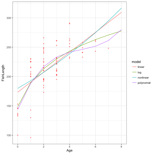

plot of chunk unnamed-chunk-5

Lets look at the distribution of the residuals of each model to the actual data. What would you expect to see?

resid_lm<-data.frame(model = "linear",resid = augment(lm_mod)$.resid)
resid_log<-data.frame(model = "log",resid = augment(log_mod)$.resid)
resid_poly<-data.frame(model = "poly",resid = augment(poly_mod)$.resid)
resid_nl<-data.frame(model = "nonlinear",resid = augment(nl_mod)$.resid)


all_resid<-rbind(resid_lm, resid_log, resid_poly, resid_nl)
head(all_resid)

##    model       resid
## 1 linear -44.3284415
## 2 linear   7.7139542
## 3 linear -12.2754468
## 4 linear  22.7033553
## 5 linear -13.3178426
## 6 linear  -0.3072437

glimpse(all_resid)

## Observations: 328
## Variables: 2
## $ model <chr> "linear", "linear", "linear", "linear", "linear", "linea...
## $ resid <dbl> -44.3284415, 7.7139542, -12.2754468, 22.7033553, -13.317...

ggplot(data = all_resid) +
  geom_violin(aes(x = model, y  =resid, fill = model)) + 
  theme_bw()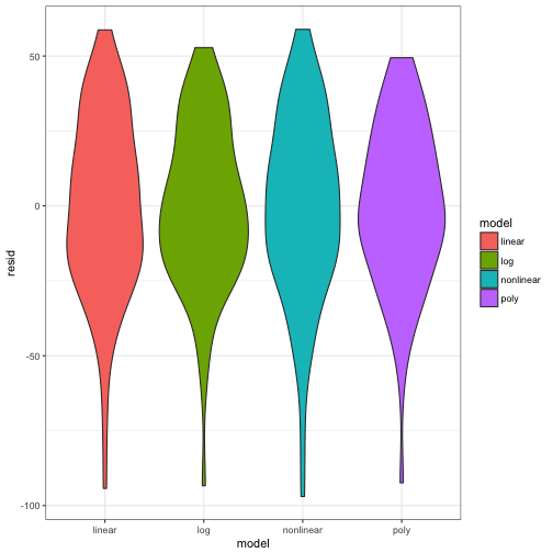

plot of chunk unnamed-chunk-6

Experiments, Events, and Probability

In probability theory, we are concerned with the occurence of events that can be thought of as outcomes of experiments
The probability of event A occurring is \( Pr { A } \) = probability that the event occurs
The Frequentist interpretation of probability \( Pr { A } \) is the proportion of A outcomes as the total number of trials in an experiment goes to infinity.

Coin flipping example:

For example, it can be demonstrated that the proportion of heads from a series of fair coin flips will approach the constant 0.5 as the number of trials grows large, that is, \( Pr { Head } \) = 0.5

## Binomial distribution
?rbinom
set.seed(12345)

N_flips<-data.frame(N = c(1:5000))
N_flips$N_heads <- unlist(lapply(lapply(N_flips$N, rbinom, size = 1, prob = 0.50), sum))
N_flips$prop <- N_flips$N_heads/N_flips$N

head(N_flips)

##   N N_heads      prop
## 1 1       1 1.0000000
## 2 2       2 1.0000000
## 3 3       1 0.3333333
## 4 4       3 0.7500000
## 5 5       1 0.2000000
## 6 6       1 0.1666667

If we look at the first 100, you can see

ggplot(data = N_flips) +
  geom_line(aes(x = N, y = prop)) + 
  geom_hline(aes(yintercept = 0.5), colour = "red", linetype = "dotted") +
  coord_cartesian(xlim = c(0, 100)) +
  theme_bw()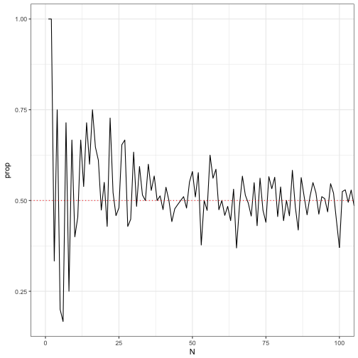

plot of chunk unnamed-chunk-8

Lets look at the whole range

ggplot(data = N_flips) +
  geom_line(aes(x = N, y = prop)) + 
  geom_hline(aes(yintercept = 0.5), colour = "red", linetype = "dotted") +
  coord_cartesian(xlim = c(0, 5000)) +
  theme_bw()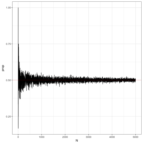

plot of chunk unnamed-chunk-9

The Bayesian interpretation of probability is the degrees of belief. For a Bayesian, \( Pr{A}\) is a measure of certainty; a quantication of an investigator’s belief that A is true.
Differences in Frequentist and Bayesian perspectives are most important pertaining to inferential procedures (e.g., parameter estimation and hypothesis testing). They are irrelevant to the mathematical principles of probability.