The Confrontation: Sum of squares

library(tidyverse)
library(broom)

Sources of the notes for this lecture are from Ecological Detective (Chapter 5).

• Simplest technique for the confrontation between models and data is sum of squares

  1. It is simple and makes few assumptions
  2. Long and successful history in science
  3. Computers can do remarkable calcualations associated with sum of squares

Basic method

Consider a simple model: $Y_i = A + BX_i = CX_i^2 + W_i$ where \(W_i\) is process uncertainty, and A, B, and C are parameters.

• For variables \(X_1, X_2, …., X_n\) we can generate predictions for Y with potential values for the parameters A, B, and C
• We can measure the deviation between the \(i^{th}\) predicted value and the \(i^{th}\) observed value: \( (Y_{pred,i} - Y_{obs,i})^2 \)
• We then sum the squared deviations to obtain a measure of fit between model and the data
• The best model (i.e., values for A, B, and C) will have the lowest sum of squares

Basic approach: Psuedocode 5.1

1. Input the data and generate a range of potential values for A, B, and C
   • Potential values should go from a minimum value to a maximum value by set increments
2. Starting at the minimum values of the parameters generate a prediction of Y for each value of X. Calculate the sum of squares
3. Compare sum of squares to the current lowest value of sum of squares, if it is less than the lowest value of sum of squares, then replace the current lowest sum of squares with the new one and the parameter values associated with the lowered sum of squares.
4. Keep going until the maximum values of the parameters have been reached.

Psuedocode 5.2

1. Specify values of the parameters A, E, and C, the number of data points to be generated, and the distribution of the process uncertainty. Set i = 1
2. Choose Xi (e.g., by systematic choice of the independent variable X).
3. Choose a particular value Wi of the process uncertainty W;.
4. Determine Yi according to Yi= A + EXi + ex? + Wi
5. Increase i by 1. If this is less than the number of data points to be generated, return to Step 2. Otherwise, stop.

set.seed(12345)

A = 1
B = 0.5
C = 0.25
X = 1:10

W = runif(10,min = -3, max = 3)
values <- data.frame(X = X, Y_determ = A + B*X + C*X^2, Y_result = A + B*X + C*X^2 + W)
values

##     X Y_determ  Y_result
## 1   1     1.75  3.075423
## 2   2     3.00  5.254639
## 3   3     4.75  6.315894
## 4   4     7.00  9.316747
## 5   5     9.75  9.488886
## 6   6    13.00 10.998231
## 7   7    16.75 15.700572
## 8   8    21.00 21.055346
## 9   9    25.75 27.116232
## 10 10    31.00 33.938422

Sum of squares

poss_A = seq(from = -1, to = 3, by = 0.1)
poss_B = seq(from = 0, to = 2, by = 0.05)
poss_C = seq(from = 0, to = 1, by = 0.025)

all_possible <- expand.grid(A = poss_A, B = poss_B, C = poss_C)
all_possible$SS <- NA
all_possible$SSW <- NA

for( i in 1:nrow(all_possible)){
  # print(i)
  pred_Y = all_possible$A[i] + all_possible$B[i]*X + all_possible$C[i]*(X^2)
  
  
  all_possible$SS[i] <- sum(pred_Y - values$Y_determ)^2
  all_possible$SSW[i] <- sum(pred_Y - values$Y_result)^2
}

id <- which(all_possible$SS == min(all_possible$SS))
all_possible[id,]

##       A   B    C SS      SSW
## 17241 1 0.5 0.25  0 72.42677

id <- which(all_possible$SSW == min(all_possible$SSW))
all_possible[id,]

##         A    B   C    SS          SSW
## 20248 2.4 0.05 0.3 72.25 0.0001079907

values$Pred_Y <- all_possible$A[id] + all_possible$B[id]*X + all_possible$C[id]*X^2

We can examine the relationship between the predicted and observed values.

ggplot(data = values) + 
  geom_point(aes(x = X, y = Y_result), size = 4, colour = "red", alpha = 0.35) +
  geom_point(aes(x = X, y = Pred_Y), size = 4, colour = "blue", alpha = 0.35) + 
  theme_bw()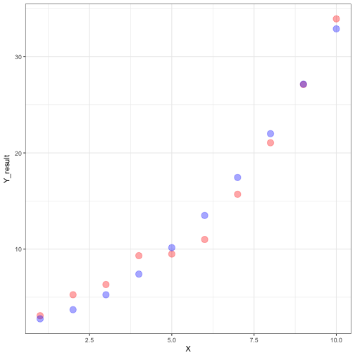

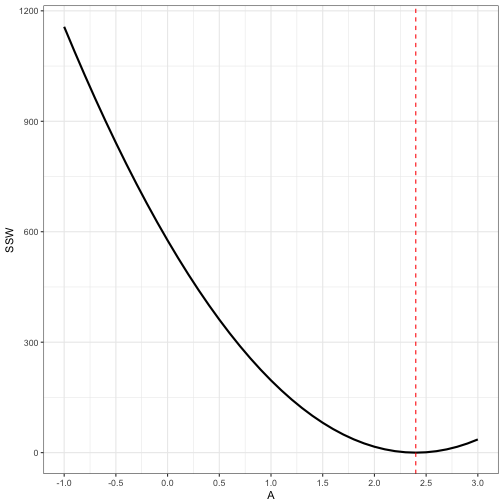
Goodness of fit

• Helpful to consider how sensitive the fit of the model and the data is to variation in the parameters.
  • Tells us how the sum of squares behaves if one of the parameters (the one that we systematically vary) is known
  • Tells us how sensitive the parameters are to one another
  • Provides some notion of confidence in our estimate of the parameter

id <- which(all_possible$B == 0.05 & round(all_possible$C,digits = 3) == 0.300)

ggplot(data = all_possible[id,]) + 
  geom_line(aes(x = A, y = SSW), size = 1) + 
  geom_vline(aes(xintercept = 2.4), colour = "red", linetype = "dashed") +
  scale_x_continuous(breaks = seq(-1,3,by = 0.5)) +
  theme_bw()