Incidental catch in fisheries: seabirds in the New Zealand squid trawl fisheries

library(tidyverse)
library(broom)

Sources of the notes for this lecture are from Ecological Detective (Chapter 4).

Motivation

Squid trawl

Non-target species are often caught during fishing operations
Observer programs are used to monitor this incidental catch
Understanding of the coverage of the program and how to interpret the data is needed

hauls = c(807, 37, 27, 8, 4, 4, 1, 3, 1, 0, 0, 2, 1, 1, 0, 0, 0, 1)  # from table 4.3
albatross = c(0:17)
incidental<-data.frame(albatross, hauls)

and let’s look at the distribution by plotting a bar chart

ggplot(data = incidental) + 
  geom_bar(aes(x= albatross, y = hauls), fill = "dodgerblue", colour = "black", stat = "identity") + 
  coord_cartesian(xlim = c(-1,18), ylim = c(0,850), expand = FALSE) + 
  theme_bw()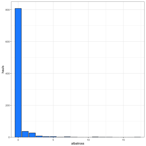

plot of chunk unnamed-chunk-3

Pseudocode 4.1

Specify the level of observer coverage, $N_{tow}$ per simulation, and the total number of simulations $N_{sim}$, and the negative binomial parameters m and k. These are estimated from last year’s data. Also specifY the criterion “success,” d, and the value of $t_q$

albatross_all <- rep(incidental$albatross, times = incidental$hauls)
length(albatross_all)

## [1] 897

albatross_mean = mean(albatross_all)

k = mean(albatross_all)^2/(var(albatross_all)- mean(albatross_all))
m <- albatross_mean
Ntows = 5000 #eventually we will increase this to 5000
iter = 150 # eventually we will increase this to 150
tq = 1.645

crit_success = 0.25*m

On the $j^{th}$ iteration of the simulation, for the ith simulated tow, generate a level of incidental take $C_{ij}$ using Equation 4.7. To do this, first generate the probability of n birds in the by-catch for an individual tow, then calculate the cumulative probability of n or fewer birds being obtained in the by-catch. Next draw a uniform random number between zero and 1, and then see where this random number falls in the cumulative distribution. Repeat this for all $N_{tow}$ tows

First generate the pdf and cdf

c = 0:100
probs <- (gamma(k + c)/(gamma(k)*factorial(c))) * ((k/(k+m))^k) * ((m/(m+k))^c)
p_c<-data.frame(c, probs)
p_c$cdf<- cumsum(p_c$probs)

ggplot(data = p_c) + 
  geom_bar(aes(x= c, y = probs), fill = "red", colour = "black", stat = "identity") + 
  coord_cartesian(xlim = c(-1,101), ylim = c(0,1), expand = FALSE) + 
  labs(x="Number of birds captured", y = "pdf") +
  theme_bw()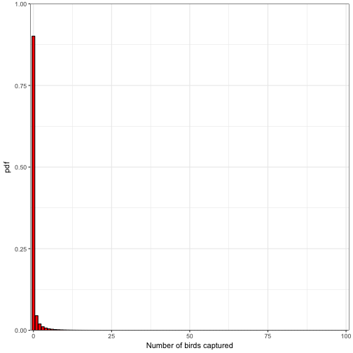

plot of chunk unnamed-chunk-5

ggplot(data = p_c) + 
  geom_bar(aes(x= c, y = cdf), fill = "green", colour = "black", stat = "identity") + 
  coord_cartesian(xlim = c(-1,101), ylim = c(0,1), expand = FALSE) + 
  labs(x="Number of birds captured", y = "cdf") +
  theme_bw()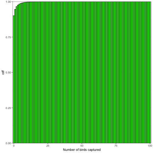

plot of chunk unnamed-chunk-5

Compute the mean

$M_j = \frac{1}{N_{tow}} \sum_{i=1}^{N_{tow}}C_{ij}$

and the variance

$S_j^2 = \frac{1}{N_{tow}-1} \sum_{i=1}^{N_{tow}}(C_{ij} - M_j)^2$

on the $j^{th}$ iteration of the simulation.

Compute the range, in analogy to Equation 4.4: $(Range)_j = 2\frac{S_j}{\sqrt{N_{tow}}}t_q$
If (Range) is less than the specified range criterion for success, increase the number of successes by 1.
Repeat steps 2-5 for j = 1 to $N_{sim}$. Estimate the probability of success when Nr.ow tows are observed by dividing the total number of successes by N_{tow}.

Start the loop. NOTE: I changed the way the loop was run from the psuedo code by nesting iterations within tows. NOTE: This simulation will take a few minutes to run. I have run the simulations ahead of time and put them up on github

set.seed(12345)

## Create a function that will allow us to more easily find the corresponding catch for each random number

find_catch <- function(pc,rand_val){
   id<-which(rand_val>=p_c$cdf)  # find which values are greater than or equal to our cdf
   id<-ifelse(length(id)<1,1,max(id))  # correct for if none are larger and otherwise take the max id
   return(p_c$c[id])
  }

tows <- seq(25,Ntows,by = 25)
s_stor <- data.frame(tows = tows, s = NA, iter = iter)

  for(i in 1:length(tows)){
    s = 0
    print(paste("Ntows = ",tows[i],sep = ""))
    for(j in 1:iter){
      # print(j)
      rand_uni<-runif(tows[i])  #generate j number of random uniform variables
      catch<- sapply(rand_uni, function(x) find_catch(pc,x)) # use the find_catch function to find the corresponding numbr of birds from our find_catch function
      
      M_j = mean(catch)  # Step 3 in the psuedo code
      S_j2 = var(catch)
      Range_j = 2*(sqrt(S_j2)/sqrt(tows[i]))*tq # Step 4 in the psuedo code

      s = ifelse(Range_j < crit_success & Range_j > 0, s+1,s) # Step 5 in the psuedo code
    }
  
    s_stor$s[i] <-s
  
  }

incidental<-s_stor

Plot the results

#  if reading from the github, otherwise comment this out if you are using your own simulation. 
incidental<-read_csv("https://raw.githubusercontent.com/chrischizinski/SNR_R_Group/master/data/incidental.csv")

## Parsed with column specification:
## cols(
##   tows = col_double(),
##   s = col_double(),
##   iter = col_double()
## )

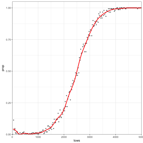
incidental$prop <- incidental$s/incidental$iter

ggplot(data = incidental) + 
  geom_point(aes(x = tows, y = prop), size = 1, alpha = 0.5) +
  geom_smooth(aes(x = tows, y = prop),method = "lm", formula = y ~ splines::bs(x, 25), colour = "red",se = FALSE) +
  coord_cartesian(ylim=c(0,1.05), xlim = c(0,5000), expand = FALSE) +
  theme_bw()

plot of chunk unnamed-chunk-7