Ecological Detective - Probability and probability models. Part 2

library(tidyverse)
library(broom)

Sources of the notes for this lecture are a combination of Aho(2013) (Chapters 2 and 3) and Ecological Detective (Chapters 3 and 4).

Common distributions

Discrete

Negative binomial distribution

Negative binomial gives the probability that x independent Bernoulli failures will occur prior to obtaining the rth success - two parameters: r is the number of successes and $ \pi $ is the probability of an individual Bernoulli success

First form:

$\mathbf{Pr(s^{th}\:success\:occurs\:on\:trial\:u + s)} = \left(\begin{array} {c} u + s -1 \\ u \end{array}\right)p^s(1-p)^u$

where: p is the probability of successes, s number of trials for success, and u is the number of not succeeding and possible values for u > 0 and 0 < p > 1.

Second form:
Assumes that the rate parameter has its own probability distribution.

$\mathbf{Pr(s^{th}\:success\:occurs\:on\:trial\:u + s)} = \left(\begin{array} {c} n + s -1 \\ s \end{array}\right)p^n(1-p)^s$

where n can be any value and not just n > 0. n is often called the “over dispersion” parameter

The mean of the negative binomial is

$E(Z(t)) = \frac{n(1-p)}{p} = \frac{n}{a}t = m(t)$

The variance of the negative binomial is $VAR(Z(t)) = m(t) + \frac{m(t)^2}{n}$

Suppose, species A has a 0.10 probability of occurring in any given plot. What is the probability of systematically exploring 0 to 150 plots to find 5 organisms, if we know the organism distribution follows a negative binomial distribution?

x <- 0:150
size <- 5
prob = 0.1
nb_data<-data.frame(x = x, size = size, pdf = dnbinom(x = x, size = size, prob = prob))

head(nb_data)

##   x size          pdf
## 1 0    5 0.0000100000
## 2 1    5 0.0000450000
## 3 2    5 0.0001215000
## 4 3    5 0.0002551500
## 5 4    5 0.0004592700
## 6 5    5 0.0007440174

Plot it

ggplot(data = nb_data) +
  geom_bar(aes(x = x, y = pdf), stat = "identity", width = 0.85) + 
  coord_cartesian(ylim = c(0,0.025), xlim = c(0, 150), expand = FALSE) +
  scale_x_continuous(breaks = seq(0,150, by = 5)) +
  theme_bw()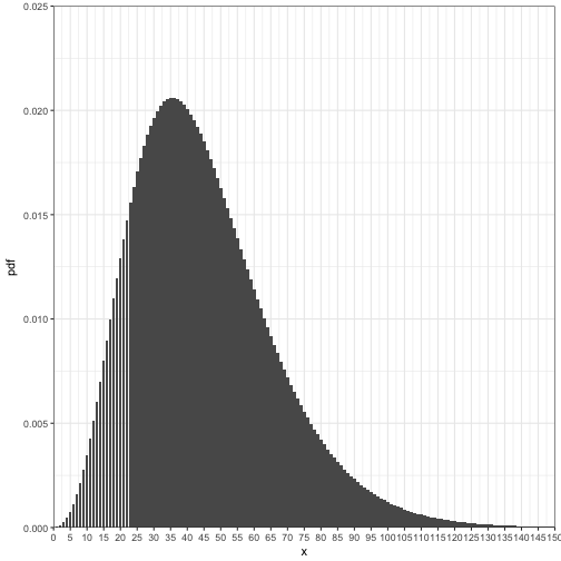

plot of chunk unnamed-chunk-3

What is the probability of finding 5 of species A in 35 plots?

sum(dnbinom(0:35, size = 5, prob = 0.10))

## [1] 0.3709823

#or
pnbinom(35, size = 5, prob = 0.10)

## [1] 0.3709823

Alternative specification uses the mean mu rather than the rate p.

From the help for dbinom():

An alternative parametrization (often used in ecology) is by the mean mu, and size, the dispersion parameter, where prob = size/(size+mu). The variance is mu + mu^2/size in this parametrization. <

Suppose, species A that it has been shown that it takes approximately 25 areas to search before you have 5 organisms. What is the probability of systematically exploring 0 to 150 plots to find 5 organisms, if we know the organism distribution follows a negative binomial distribution with a mean of 25?

x <- 0:150
size <- 5
mu = 25
nb_data2<-data.frame(x = x, size = size, pdf = dnbinom(x = x, size = size, mu = mu))

ggplot(data = nb_data2) +
  geom_bar(aes(x = x, y = pdf), stat = "identity", width = 0.85) + 
  coord_cartesian(ylim = c(0,0.04), xlim = c(0, 150), expand = FALSE) +
  scale_x_continuous(breaks = seq(0,150, by = 5)) +
  theme_bw()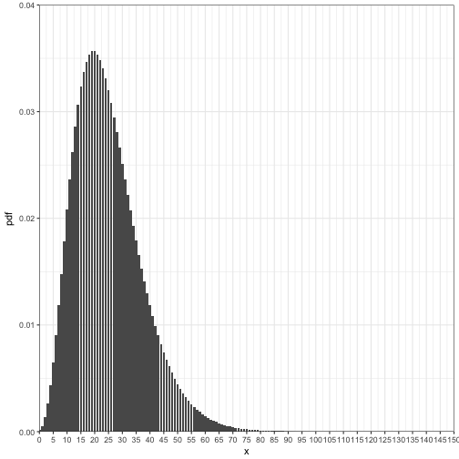

plot of chunk unnamed-chunk-5

Continuous

Normal or Gaussian

Most commonly used continuous pdf in statistics is the normal distribution or Gaussian distribution
It is used to represent processes where the most likely outcome is the average and it is symmetric around the average
Two parameters are $ \mu $ mean and $ \sigma $ standard deviation
expected outcomes for $ x \in {\rm I\!R} $ and $ \sigma > 0 $

Standard normal or Z-distribution

$ \mu = 0$ and $ \sigma = 1 $

Suppose the mean tarsus length of an adult pheasant is 72.5 mm and the standard deviation is 2.36. Assuming this follows a normal distribution, construct a pdf from 60 mm to 85 mm.

x<- seq(60,85, by = 0.01)
sd = 2.36
mu = 72.5

nrm_data<-data.frame(x = x, sd = sd, mean = mu, pdf = dnorm(x = x, mean = mu, sd = sd))

head(nrm_data)

##       x   sd mean             pdf
## 1 60.00 2.36 72.5 0.0000001368145
## 2 60.01 2.36 72.5 0.0000001399185
## 3 60.02 2.36 72.5 0.0000001430904
## 4 60.03 2.36 72.5 0.0000001463316
## 5 60.04 2.36 72.5 0.0000001496434
## 6 60.05 2.36 72.5 0.0000001530275

and plot it out.

ggplot(data = nrm_data) +
  geom_line(aes(x = x, y = pdf)) + 
  coord_cartesian(ylim = c(0,0.20), xlim = c(60, 85), expand = FALSE) +
  labs(x = "Tarsus length", y = "density") +
  theme_bw()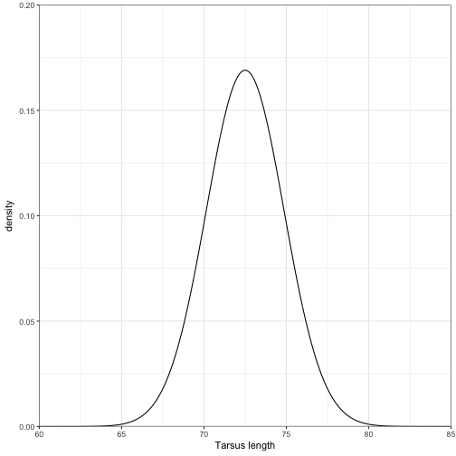

plot of chunk unnamed-chunk-7

What is the probability that the tarsus length is at least 68 mm?

sd_away <- ((68 - mu)/sd) 
norm_function<-function(x){1/sqrt(2 * pi) * exp(-1/2 * x^2)}

integrate(norm_function, lower= -Inf, upper=sd_away)

## 0.02827456 with absolute error < 0.000025

#or

integrate(dnorm,-Inf, sd_away)

## 0.02827456 with absolute error < 0.000025

# or
pnorm(sd_away)

## [1] 0.02827456

What is the probability that the tarsus length is between 68 mm and 70 mm?

sd_away1 <- ((68 - mu)/sd) 
sd_away2 <- ((70 - mu)/sd) 


integrate(dnorm,sd_away1, sd_away2)

## 0.116452 with absolute error < 1.3e-15

ggplot(data = nrm_data) +
  geom_ribbon(data = nrm_data[nrm_data>= 68 & nrm_data <=70, ],aes(x = x, ymin = 0, ymax = pdf), fill = "lightblue") +
  geom_line(aes(x = x, y = pdf)) +
  coord_cartesian(ylim = c(0,0.20), xlim = c(60, 85), expand = FALSE) +
  labs(x = "Tarsus length", y = "density") +
  theme_bw()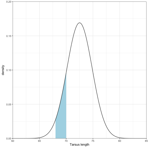

plot of chunk unnamed-chunk-9

Lognormal distribution

If a random variable X has a log normal distribution, and Y = log(X), then Y will have a normal distribution.

Correspondingly, if Y is normally distributed then $ e^Y $ will be lognormally distributed.

Two parameters are $ \mu $ location parameter and $ \sigma $ scale parametre
expected outcomes for $ \mu \in {\rm I\!R} $ and $ \sigma > 0 $
Many variables in biology have lognormal distributions (cannot be less than zero, are right-skewed) and are normally distributed after log-transformation

ln_data <- data.frame(x = c(0:15), 
                      pdf1 = dlnorm(x = c(0:15), meanlog = 0, sdlog = 1),
                      pdf2 = dlnorm(x = c(0:15), meanlog = 0, sdlog = 5),
                      pdf3 = dlnorm(x = c(0:15), meanlog = 2, sdlog = 1)
                      )

ggplot(data = ln_data) +
  geom_line(aes(x = x, y = pdf1) ,colour = "red", size = 1) +
  geom_line(aes(x = x, y = pdf2) ,colour = "blue", size = 1) +
  geom_line(aes(x = x, y = pdf3) ,colour = "purple", size = 1) +
  coord_cartesian(ylim = c(0,0.50), xlim = c(0,15), expand = FALSE) +
  labs(x = "X", y = "density") +
  theme_bw()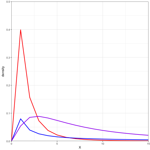

plot of chunk unnamed-chunk-10

Chi-square distribution

The $ \chi^2 $ is defined by the degrees of freedom (the number of independent pieces of information that exist concerning an estimable parameter)
The $ \chi^2 $ distribution is frequently used for testing the null hypothesis that observed and expected frequencies are equal
The $ \chi^2 $ distribution results from the summing of independent, squared, standard normal distributions
Has the following form: $f(x) = \frac{1}{2^{v/2}\Gamma(v/2)}x^{(v/2)-1}e^{-x/2}$
- where outcomes are continuous and independent, $x \geq 0 $, $v \geq 0 $, and $ \Gamma(.) $ is the gamma function.
- $ \Gamma(x)= (x-1)!$

x = 6
factorial(x - 1)

## [1] 120

gamma(x)

## [1] 120

Let’s explore the relationship between the standard normal and the $ \chi^2 $ distribution by generating 10000 standard random normal values. We will then $ x^2 $ thos values and compare the distributions.

set.seed(12345)

#generate standard normal
rand.data<-data.frame(std_norm = rnorm(10000))

# plot the density of those values
ggplot(data = rand.data) + 
  geom_density(aes(x = std_norm), fill = "lightblue") +
  coord_cartesian(xlim = c(-4,4), ylim = c(0,0.5), expand = FALSE) +
  theme_bw()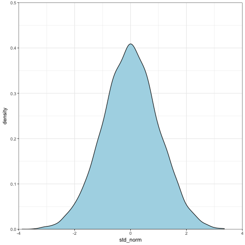

plot of chunk unnamed-chunk-12

# square our standard normal
rand.data$chi <- rand.data$std_norm^2

# plot the density of those values
ggplot(data = rand.data) + 
  geom_density(aes(x = chi), fill = "red") +
  coord_cartesian(xlim = c(0,15), ylim = c(0,1.25), expand = FALSE) +
  annotate("text", x = 5, y = 0.75, parse = T, label = as.character(expression(paste(~chi^2,"distribution with 1 df"))), size = 6, hjust = 0.2) +
  theme_bw()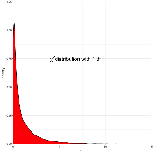

plot of chunk unnamed-chunk-12

The degrees of freedom is equal to the $ \mu $, variance is equal to 2*df, and mode is df - 2

Lets look at the $ \chi^2 $ distribution with varying degrees of freedom.

x = 0:25
chi_data <- data.frame(x = x,
                       df1 = dchisq(x,1),
                       df3 = dchisq(x,3),
                       df6 = dchisq(x,6),
                       df12 = dchisq(x,12))

chi_data %>% 
  gather(df, value, df1:df12) %>% 
  mutate(df = factor(df, levels = c("df1","df3","df6","df12"))) -> chi_data

ggplot(data = chi_data) +
  geom_line(aes(x = x, y = value, colour = df, group = df), size = 1) + 
  coord_cartesian(xlim = c(0,25), ylim = c(0,0.25), expand = FALSE) +
  theme_bw()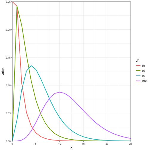

plot of chunk unnamed-chunk-13

Gamma distribution

The gamma distribution is named after the gamma functioned described above.
$ \theta$ is the scale parameter and $ \kappa$ is the shape parameter
Outcomes are continuous and independent, x > 0 and $ \theta >0$, $ \kappa >0$
The mean is $ \theta * \kappa $
The gamma distribution is most frequently used for representing phenomena with highly right-skewed probability distributions
- However it is extremely flexible and can be used to mimic other pdfs

x = 0:30
gamm_data <- rbind(data.frame(type = "vary shape", scale = 5, shape = 1, x = x, y =  dgamma(x = x, shape = 1, scale = 2)),
                   data.frame(type = "vary shape",scale = 5, shape = 10, x = x, y =  dgamma(x = x, shape = 2, scale = 2)),
                   data.frame(type = "vary shape",scale = 5, shape = 20, x = x, y =  dgamma(x = x, shape = 3, scale = 2)))
                   

gamm_data2 <- rbind(data.frame(type = "vary scale",scale = 1, shape = 10, x = x, y =  dgamma(x = x, shape = 2, scale = 1)),
                   data.frame(type = "vary scale",scale = 5, shape = 10, x = x, y =  dgamma(x = x, shape = 2, scale = 2)),
                   data.frame(type = "vary scale",scale = 10, shape = 10, x = x, y =  dgamma(x = x, shape = 2, scale = 3)))

all_gamm_data <- rbind(gamm_data, gamm_data2)
all_gamm_data$type <- factor(all_gamm_data$type, levels = c("vary shape", "vary scale"))
                   
                   
ggplot(data = all_gamm_data) +
  geom_line(aes(x = x, y = y, colour = paste(scale, shape), group = paste(scale, shape)), size = 1) + 
  coord_cartesian(xlim = c(0,30), ylim = c(0,0.5), expand = FALSE) +
  scale_x_continuous(breaks = seq(0,30, by = 5)) +
  facet_wrap(~type) +
  theme_bw()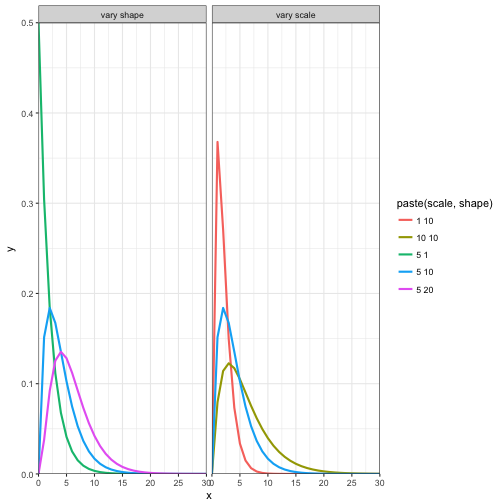

plot of chunk unnamed-chunk-14

Monte Carlo Methods

In order to confront models with data, we need to estimate parameters and choose one description over another
In most cases, we do not know the underlying mechanisms and processes
One way to test our confidence in our models is to test models on sets of simulated data that we construct with known mechanisms and processes (Monte Carlo or stochastic simulation)
Monte Carlo methods uses random-number generators to construct data
One type of random number generator is the random uniform (runif() in R) that generates continuous values between a minimum (usually 0) and maximum (usually 1) where probability of each value being drawn is equal
Other distributions inclue: binomial (rbinom() in R), Poisson (rpois() in R), negative binomial (rnbinom() in R), normal (rnorm() in R), gamma (rgamma() in R), and many others

Ecological scenarios: Simple population model with process and observation uncertainty

** What are the differences between process and observation uncertainty? **

We can use Monte Carlo simulations to explore process and observation uncertainty in a simple population model

$N_{t +1} = sN_t + b_t + W_t$ $N_{obs,t} = N_t + V_t$

#Psuedocode 3.4
set.seed(54321)

s = 0.8
b = 20
N0 = 50 
sig_w = 10 # process uncertainty, random normal with mean 0 and sd = 10
sig_v = c(0,10) # observation uncertainty, random normal with mean 0 and sd 0 and 10

Nt = N0
t_total = 50 + 1

N_stor <- as.data.frame(matrix(0, t_total,3))
names(N_stor) <- c("Nt", "Nobs0", "Nobs10")

for(t in 1:t_total){
  N_stor$Nt[t]<-Nt # Place the population number at time t in  N_stor
  Nt_1 = s*Nt + b + rnorm(1,mean = 0, sd = sig_w) # Calculate the population at t + 1
  N_obs0 = Nt + rnorm(1,mean = 0, sd = sig_v[1]) # Calculate observation error (none)
  N_stor$Nobs0[t]<-N_obs0 # Place the observed population number at time t in  N_stor 
  N_obs10 = Nt + rnorm(1,mean = 0, sd = sig_v[2]) # Calculate observation error (none)
  N_stor$Nobs10[t]<-N_obs10 # Place the observed population number at time t in  N_stor 
  Nt <- Nt_1 # change Nt to Nt+1
  }

head(N_stor)

##         Nt    Nobs0   Nobs10
## 1 50.00000 50.00000 40.71956
## 2 58.21099 58.21099 41.70499
## 3 58.72846 58.72846 47.77316
## 4 62.90210 62.90210 88.06256
## 5 53.39926 53.39926 55.19903
## 6 76.67293 76.67293 89.31436

Lets look a plot of population at time t and population at t + 1 (Figure 3.6)

lagged_data<-data.frame(Nt =N_stor$Nt[-51], Nt_1 = N_stor$Nt[-1])

lm_mod<- lm(Nt~Nt_1, data = lagged_data)
summary(lm_mod)

## 
## Call:
## lm(formula = Nt ~ Nt_1, data = lagged_data)
## 
## Residuals:
##      Min       1Q   Median       3Q      Max 
## -24.8374  -7.2374  -0.5361   7.4813  24.4717 
## 
## Coefficients:
##             Estimate Std. Error t value Pr(>|t|)    
## (Intercept) 15.55382    8.13203   1.913   0.0618 .  
## Nt_1         0.81754    0.09155   8.930 8.98e-12 ***
## ---
## Signif. codes:  0 '***' 0.001 '**' 0.01 '*' 0.05 '.' 0.1 ' ' 1
## 
## Residual standard error: 10.93 on 48 degrees of freedom
## Multiple R-squared:  0.6243,	Adjusted R-squared:  0.6164 
## F-statistic: 79.75 on 1 and 48 DF,  p-value: 8.979e-12

newdata <- data.frame(Nt_1 = 0:160)

pred_mod <- augment(lm_mod, newdata = newdata) 

ggplot(data = lagged_data) + 
  geom_line(data = pred_mod, aes(x = Nt_1, y = .fitted), linetype = "dashed") + 
  geom_point(aes(x = Nt_1, y = Nt), size = 2, shape = 1, colour = "red") + 
  coord_cartesian(ylim = c(0, 150), xlim = c(0, 150), expand = FALSE) +
  labs(x = "Population size at time t + 1", y = "Population size at time t") +
  theme_bw()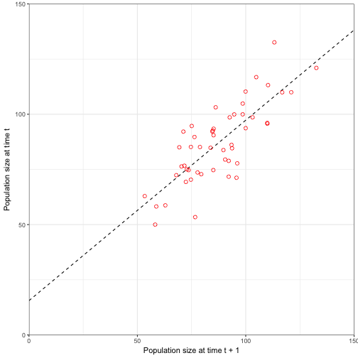

plot of chunk unnamed-chunk-16

We can see in this figure that the process uncertainty (remember we did not look at observation uncertainty) influences the values by scattering the points along the mean (regression line). However, there is still a strong relationship between the two values (($R^2$ = 0.6242727)). We can see that the birth rate (15.5538219) is close to our birth rate (20) and the survival rate (0.8175352) is close to our survival rate (0.8).

Now let’s look at the influence of observation uncertainty with a plot of observed population at time t and observed population at t + 1 (Figure 3.7)

lagged_data2<-data.frame(Nobs10 =N_stor$Nobs10[-51], Nobs10_1 = N_stor$Nobs10[-1])

lm_mod2<- lm(Nobs10~Nobs10_1, data = lagged_data2)
summary(lm_mod2)

## 
## Call:
## lm(formula = Nobs10 ~ Nobs10_1, data = lagged_data2)
## 
## Residuals:
##    Min     1Q Median     3Q    Max 
## -39.61 -15.56   3.88  12.54  31.26 
## 
## Coefficients:
##             Estimate Std. Error t value  Pr(>|t|)    
## (Intercept)  35.7564    11.2686   3.173   0.00263 ** 
## Nobs10_1      0.5863     0.1251   4.685 0.0000233 ***
## ---
## Signif. codes:  0 '***' 0.001 '**' 0.01 '*' 0.05 '.' 0.1 ' ' 1
## 
## Residual standard error: 17.55 on 48 degrees of freedom
## Multiple R-squared:  0.3138,	Adjusted R-squared:  0.2995 
## F-statistic: 21.95 on 1 and 48 DF,  p-value: 0.00002334

newdata <- data.frame(Nobs10_1 = 0:160)

pred_mod2 <- augment(lm_mod2, newdata = newdata) 

ggplot(data = lagged_data2) + 
  geom_line(data = pred_mod2, aes(x = Nobs10_1, y = .fitted), linetype = "dashed") + 
  geom_point(aes(x = Nobs10_1, y = Nobs10), size = 2, shape = 1, colour = "blue") + 
  coord_cartesian(ylim = c(0, 150), xlim = c(0, 150), expand = FALSE) +
  labs(x = "Observed population size at time t + 1", y = "Observed population size at time t") +
  theme_bw()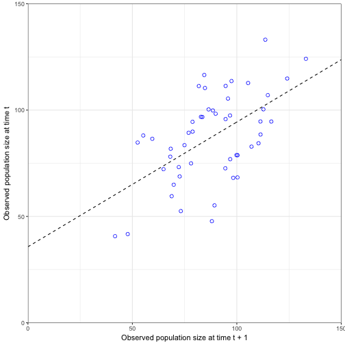

plot of chunk unnamed-chunk-17

We can see in this figure that the process uncertainty and observation uncertainty we start getting a much weaker relationship ($R^2$ = 0.3138051) by scattering the points even more along the mean. We also see that the birth rate (35.7563572) is off from our specified birth rate (20), as is the survival rate (0.5862988) compared to our specified survival rate (0.8).