library(tidyverse)Classical Probability
Sources of the notes for this lecture are a combination of Aho(2013) (Chapters 2 and 3) and Ecological Detective (Chapters 3 and 4).
- As we become familiar with the behavior of random variables, we may become aware of probabilistic patterns
Disjoint
If two events can not occur simultaneously, then we call them mutually exclusive or disoint
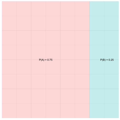
If for two outcomes A and B, we wanted to know the probability of the event A or B (expressed as: \(P( A \cup B) = P(A) + P(B) \))
We can also think of events that are not mutually exclusive. Suppose an organism has a probability of being in a habitat with environmental variable A with P = 0.3 and a habitat with environmental variable B with P = 0.3 and habitat with environmental variable A and B with P = 0.09
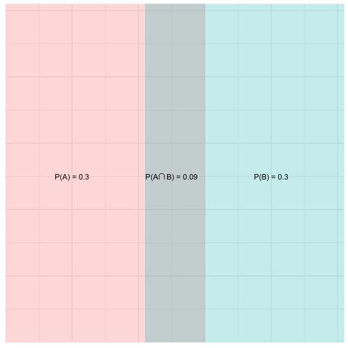
If A and B are not mutually exclusive we can sill calcualte the union of A and B as \(P( A \cup B) = P(A) + P(B) - P( A \cap B)\))
Independence
- When event A occurs it does not affect the probability of B, then we say that A and B are independent.
Conditional probability
- There can be many events that are not independent
- Suppose A is the outcome of a prey organism surviving a predator experiment on day 1 and B is the outcome of the same prey organism surviving the predator experiment the next day. If the the prey can learn and alter it’s behavior on day 1 then the outcome on day 2 is not independent. We can denote this as \( P(B|A)\) or the probability of B given A
Odds
- Closely related to probability
- The ratio between the number of favorable outcomes to the number of unfavorable outcomes. The odds of rolling a two on a dice are 1:5. Total number of outcomes = 6, Number of favorable outcomes = 1, and unfavorable outcomes (6-1) = 5.
Odds ratio and relative risk
- Ratio of the odds for two outcomes is their odds ratio
- Ratio of the probability of two events is relative risk
Probability density functions
- A probability distribution assigns probabilities to outcomes from a random variable
- The mathematical expression \(f(x)\) that defines a probability distribution is called a probability density function or pdf
- The output of the pdf is called density
Example
rand_vals<-data.frame(x = rnorm(10000))

ggplot(rand_vals) +
  geom_histogram(aes(x = x), fill = "red", colour = "black", binwidth = 1) +
  theme_bw()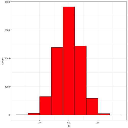
ggplot(rand_vals) +
  geom_histogram(aes(x = x), fill = "red", colour = "black", binwidth = 0.25) +
  theme_bw()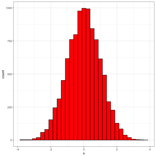
ggplot(rand_vals) +
  geom_histogram(aes(x = x), fill = "red", colour = "black", binwidth = 0.05) +
  theme_bw()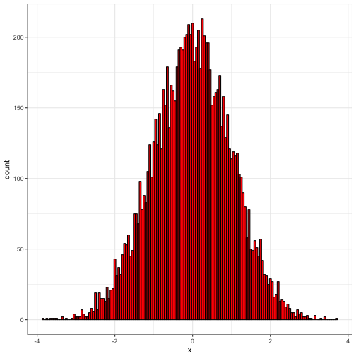
#  Add a density curve
ggplot(rand_vals,aes(x = x)) +
  geom_histogram(aes(y = ..density..), fill = "red", colour = "black", binwidth = 0.05) +
  geom_density(size = 2, colour = "blue") +
  theme_bw()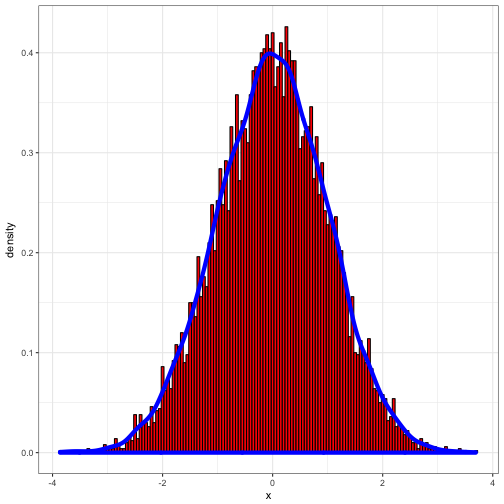
- Both discrete and continuous pdfs calculate a quantity called density.
- The “height” of any pdf “curve” at an outcome x will equal the density of x, given as \( f(x) \)
- Density is equivalent to probability for a discrete pdf, but not for a continuous pdf.
Cumulative density functions
- Cumulative distribution function (cdf) for a random variable X is denoted \(F(x)\).
- cdf is obtained by summing (discrete) or integrating (continuous) the pdf between \(-\inf\) and an outcome x
- cdf gives the lower tail probability \( P(X \leq x) \) for the both discrete and continuous random variables.
Common distributions
Discrete
Binomial
- The binomial distribution defines the probability of a particular number of successes given n independent and identically distributed Bernoulli trials
- two parameters: the number of trials (n) and the probability of success for a single trial ( \( \pi \))
Psuedo code 3.1
p = 0.1
N = 10

P_N = (1-p)^N

psuedo_dat <- data.frame(k = 1:N)
psuedo_dat$P_N <- (factorial(N)/(factorial(psuedo_dat$k)*factorial((N - psuedo_dat$k)))) * (p^psuedo_dat$k)*(1-p)^(N -psuedo_dat$k)
psuedo_dat$P_1 <- dbinom(x = 1:10, size = 10, p = 0.1)
psuedo_dat$P_2 <- dbinom(x = 1:10, size = 10, p = 0.2)
psuedo_dat$P_3 <- dbinom(x = 1:10, size = 10, p = 0.3)

psuedo_dat %>%
  select(k, P_1:P_3) %>%
  gather(probability, value, P_1:P_3) -> psuedo_dat.long

ggplot(psuedo_dat.long) +
  geom_bar(aes(x = k, y = value, fill = probability, group = probability), stat = "identity", width = 0.75, position = "dodge") +
  coord_cartesian(ylim = c(0,0.40), xlim = c(0, 10), expand = FALSE) +
  scale_x_continuous(breaks = 1:10) +
  labs(y="density",x = "Number of fruit sampled") +
  theme_bw()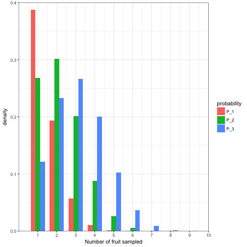
Poisson distribution
- Poisson distribution is functionally similar to the binomial distribution
- the distribution gives the probability for a defined number of successes, x, given a series of independent trials.
- As number of trials goes to infinity, the Poisson pdf will be equivalent to the binomial pdf
- No explicit maximum value for x because the Poisson distribution considers successes in the context of a fixed success rate instead of a fixed sample size (binomial)
- One variable \( \lambda \) is the mean and variance, calculated as r (rate of succcesses) * t (unit of time)
Psuedo Code 3.2
Suppose the rate parameter r is 0.5 (probability a bird flys by in a given minute) and we want to watch over time t is 10. Given that we have and r of 0.5 and we will watch for t = 10, then we would expect that approximately 5 birds would fly by mu = r*t.
r = 0.5
t = 10
cutoff = 1 - 1e-9

sum_val <- exp(-r*t)

k = 1
pois_stor<-NULL

while(sum_val <= cutoff){

  p_kt<-((exp(-r * t) * (r*t)^k)/factorial(k))

  pois_stor<-rbind(pois_stor,data.frame(k = k, p_kt = p_kt))

  sum_val = sum_val +p_kt

  k<- k +1

}

# Final K
k
## [1] 24# Final p_kt
p_kt## [1] 3.107014e-09pois_stor## k p_kt
## 1 1 3.368973e-02
## 2 2 8.422434e-02
## 3 3 1.403739e-01
## 4 4 1.754674e-01
## 5 5 1.754674e-01
## 6 6 1.462228e-01
## 7 7 1.044449e-01
## 8 8 6.527804e-02
## 9 9 3.626558e-02
## 10 10 1.813279e-02
## 11 11 8.242177e-03
## 12 12 3.434240e-03
## 13 13 1.320862e-03
## 14 14 4.717363e-04
## 15 15 1.572454e-04
## 16 16 4.913920e-05
## 17 17 1.445271e-05
## 18 18 4.014640e-06
## 19 19 1.056484e-06
## 20 20 2.641211e-07
## 21 21 6.288597e-08
## 22 22 1.429227e-08
## 23 23 3.107014e-09Or we can use dpois
pois_stor$p_kt1 <- dpois(1:23, r*t, log = FALSE)

ggplot(pois_stor) +
  geom_bar(aes(x = k, y = p_kt1), stat = "identity", width = 0.75, fill = "lightblue") +
  coord_cartesian(ylim = c(0,0.20), xlim = c(0, 23), expand = FALSE) +
  scale_x_continuous(breaks = 1:23) +
  labs(y="density",x = "k") +
  theme_bw()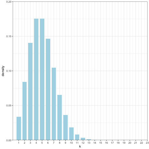
Calculate the cdf
pois_stor$cdf_kt1 <-cumsum(pois_stor$p_kt1)
pois_stor
## k p_kt p_kt1 cdf_kt1
## 1 1 3.368973e-02 3.368973e-02 0.03368973
## 2 2 8.422434e-02 8.422434e-02 0.11791407
## 3 3 1.403739e-01 1.403739e-01 0.25828797
## 4 4 1.754674e-01 1.754674e-01 0.43375534
## 5 5 1.754674e-01 1.754674e-01 0.60922271
## 6 6 1.462228e-01 1.462228e-01 0.75544552
## 7 7 1.044449e-01 1.044449e-01 0.85989038
## 8 8 6.527804e-02 6.527804e-02 0.92516842
## 9 9 3.626558e-02 3.626558e-02 0.96143400
## 10 10 1.813279e-02 1.813279e-02 0.97956678
## 11 11 8.242177e-03 8.242177e-03 0.98780896
## 12 12 3.434240e-03 3.434240e-03 0.99124320
## 13 13 1.320862e-03 1.320862e-03 0.99256406
## 14 14 4.717363e-04 4.717363e-04 0.99303580
## 15 15 1.572454e-04 1.572454e-04 0.99319304
## 16 16 4.913920e-05 4.913920e-05 0.99324218
## 17 17 1.445271e-05 1.445271e-05 0.99325664
## 18 18 4.014640e-06 4.014640e-06 0.99326065
## 19 19 1.056484e-06 1.056484e-06 0.99326171
## 20 20 2.641211e-07 2.641211e-07 0.99326197
## 21 21 6.288597e-08 6.288597e-08 0.99326203
## 22 22 1.429227e-08 1.429227e-08 0.99326205
## 23 23 3.107014e-09 3.107014e-09 0.99326205And plot the cdf
ggplot(pois_stor) +
  geom_bar(aes(x = k, y = cdf_kt1), stat = "identity", width = 0.75, fill = "lightblue") +
  coord_cartesian(ylim = c(0,1), xlim = c(0, 23), expand = FALSE) +
  scale_x_continuous(breaks = 1:23) +
  labs(y="cumulative density",x = "k") +
  theme_bw()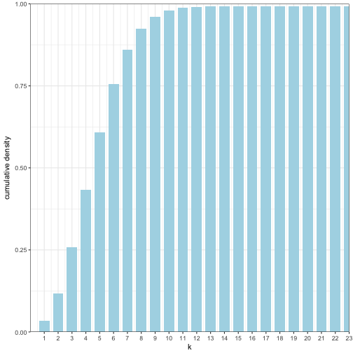
What is the probability of 4 birds flying by in 10 minutes?
sum(dpois(0:4, r*t, log = FALSE))## [1] 0.4404933ppois(4, r*t)## [1] 0.4404933