Survey Design Toolbox: Planning, Comparing, and Combining Designs

This vignette collects three M014 tools into one practitioner-facing workflow:

power_creel() for pre-season sample-size and power planning
compare_designs() for side-by-side comparison of completed survey estimates
as_hybrid_svydesign() for combining access-point and roving count data in a single survey design

library(tidycreel)

1 Pre-season sample-size planning with `power_creel()`

Pre-season planning usually starts with pilot information: expected effort by stratum, variability in daily counts, and rough interview-level CV values for catch and effort. power_creel() provides one interface for three planning questions.

Required sampling days for total effort precision

This first example estimates how many sampling days are needed in weekday and weekend strata to target a 20% RSE on the seasonal effort estimate.

effort_plan <- power_creel(
  mode = "effort_n",
  target_rse = 0.20,
  strata = c("weekday", "weekend"),
  N_h = c(90, 30),
  ybar_h = c(42, 68),
  s2_h = c(196, 441)
)

effort_plan
#>   stratum n_required target_rse
#> 1 weekday          3        0.2
#> 2 weekend          1        0.2
#> 3   total          3        0.2

The result returns one row per stratum plus a total row, making it easy to translate a seasonal precision target into a day-allocation plan.

Required interviews for CPUE precision

If the planning question is interview effort rather than count days, mode = "cpue_n" solves for the number of interviews needed to estimate CPUE with a target RSE.

cpue_plan <- power_creel(
  mode = "cpue_n",
  target_rse = 0.15,
  cv_catch = 0.85,
  cv_effort = 0.55,
  rho = 0.35
)

cpue_plan
#>   n_required target_rse cv_catch cv_effort  rho
#> 1         32       0.15     0.85      0.55 0.35

This is useful when interview staffing is the main operational bottleneck and pilot data already suggest the variability of catch and angler effort.

Power to detect a management-relevant CPUE change

The third mode asks a different question: if we can complete a fixed number of interviews, how much power do we have to detect a change in CPUE from one season to the next?

power_plan <- power_creel(
  mode = "power",
  n = 120L,
  cv_historical = 0.42,
  delta_pct = 0.20
)

power_plan
#>       power   n delta_pct cv_historical alpha alternative
#> 1 0.9580589 120       0.2          0.42  0.05   two.sided

Here delta_pct = 0.20 means a 20% change in CPUE. Together, the three modes cover the most common pre-season planning decisions: how many days to sample, how many interviews to complete, and what power that design can deliver.

2 Comparing finished designs with `compare_designs()`

Once a survey has been completed, compare_designs() helps compare multiple creel_estimates objects on a common scale. In this example we estimate total effort twice from the same dataset, changing only the variance method.

data("example_counts")
data("example_interviews")

calendar <- unique(example_counts[, c("date", "day_type")])

design <- creel_design(calendar, date = date, strata = day_type)
design <- add_counts(design, example_counts)
design <- add_interviews(
  design,
  example_interviews,
  catch = catch_total,
  effort = hours_fished,
  trip_status = trip_status,
  n_anglers = n_anglers
)

set.seed(123)

effort_taylor <- estimate_effort(design, variance = "taylor")
effort_bootstrap <- estimate_effort(design, variance = "bootstrap")

design_comparison <- compare_designs(
  list(
    Taylor = effort_taylor,
    Bootstrap = effort_bootstrap
  )
)

design_comparison
#> 
#> ── Survey Design Comparison ────────────────────────────────────────────────────
#> 2 row(s), 2 design(s)
#> 
#>      design estimate   se    rse ci_lower ci_upper ci_width  n
#> 1    Taylor      372 13.2 0.0354      344      401     57.4 14
#> 2 Bootstrap      372 13.5 0.0363      343      402     58.9 14

Because both estimates come from the same counts and interviews, the point estimate is identical while the uncertainty metrics reflect the different variance estimators.

ggplot2::autoplot(design_comparison)
#> `height` was translated to `width`.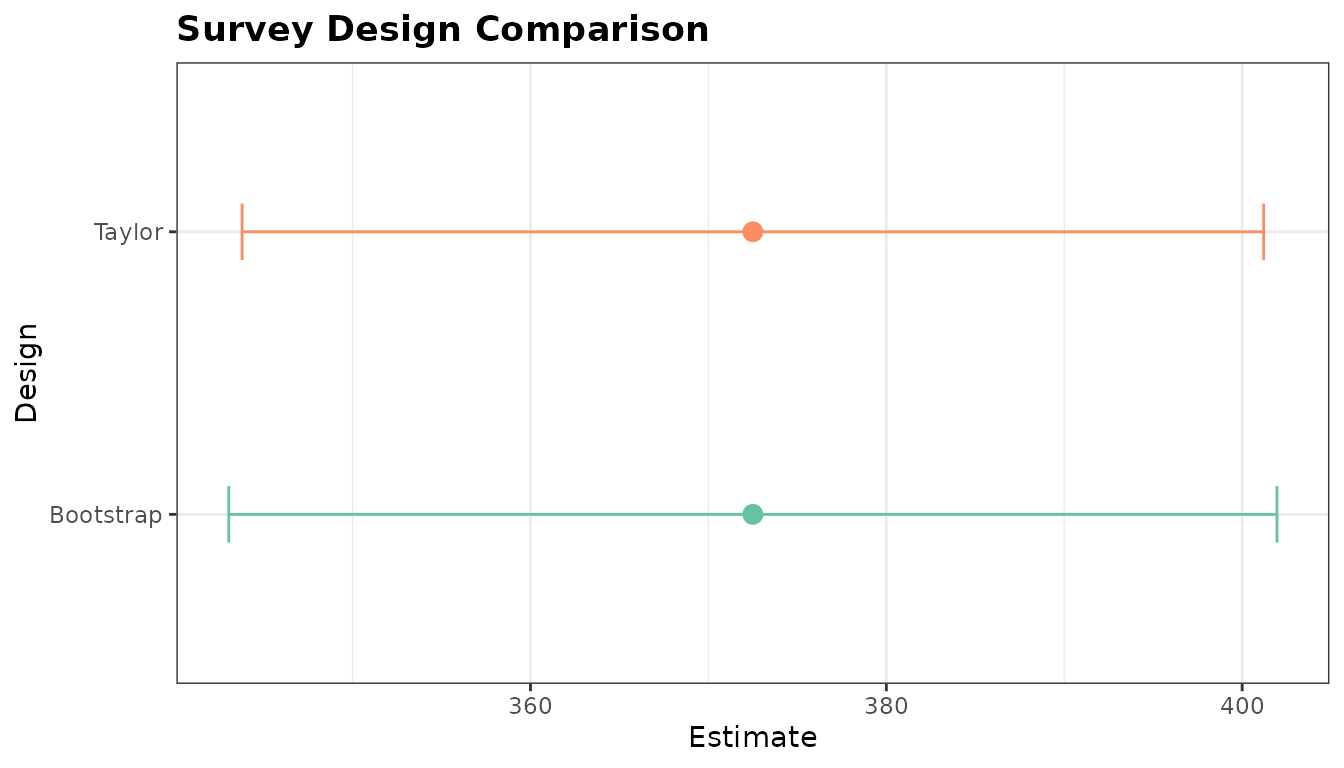

Design comparison across two effort estimators.

This pattern is helpful after a season when you want to compare alternative estimation choices without rebuilding custom summary tables by hand.

3 Combining access and roving counts with `as_hybrid_svydesign()`

Some programs collect counts from both fixed access points and roving routes. as_hybrid_svydesign() stacks those components into a single survey design object with component-specific weights.

access <- data.frame(
  date = as.Date(c("2024-06-03", "2024-06-08", "2024-06-10", "2024-06-15")),
  day_type = c("weekday", "weekend", "weekday", "weekend"),
  count = c(12L, 18L, 9L, 21L)
)

roving <- data.frame(
  date = as.Date(c("2024-06-03", "2024-06-08", "2024-06-10", "2024-06-15")),
  day_type = c("weekday", "weekend", "weekday", "weekend"),
  count = c(10L, 16L, 8L, 19L)
)

hybrid_design <- as_hybrid_svydesign(
  access_data = access,
  roving_data = roving,
  access_fraction = c(weekday = 0.5, weekend = 0.5),
  roving_fraction = c(weekday = 0.5, weekend = 0.5)
)

hybrid_design
#> 
#> ── Hybrid Creel Survey Design ──────────────────────────────────────────────────
#> Components: "access" (4 obs) + "roving" (4 obs)
#> 
#> Stratified Independent Sampling design
#> survey::svydesign(ids = ids_formula, strata = strata_formula, 
#>     weights = weights_formula, fpc = ~fpc_val, data = combined)

With the combined design in hand, standard survey estimators work directly on the stacked data.

survey::svytotal(~count, hybrid_design)
#>       total     SE
#> count   226 7.6158

This small example is intentionally self-contained, but the same pattern scales to real field programs where access and roving counts represent complementary views of the same sampling frame.

Summary

The survey-design toolbox supports the full planning-to-reporting arc:

power_creel() helps set realistic pre-season sample sizes and power targets
compare_designs() turns alternative estimator outputs into a tidy, directly comparable object with a plotting method
as_hybrid_svydesign() bridges mixed access-point and roving count programs into one survey design for downstream analysis

Used together, these tools make it easier to justify sampling effort before the season, evaluate estimator trade-offs afterward, and support hybrid monitoring programs with standard survey workflows.

1 Pre-season sample-size planning with power_creel()